Final project
Part A: Neural Fields
As a starting exercise, we can fit a neural radiance field (NeRF) on 2D images. The NeRF, $F_{\theta}: (u, v) \rightarrow (r, g, b)$, is parameterized by a multi-layer network with sinusoidal positional encoding. It maps a pixel $(u, v)$ to an RGB value $(r, g, b)$. The detailed architecture is shown in Figure 1.

Figure 1: Neural Field Architecture.
The input $x$ is a list of pixel coordinates with shape $[HW, 2]$. We randomly sampled $N$ points and normalized the pixel coordinates before passing them into the positional encoding layer. The positional encoding layer maps $x$ to a vector of shape $[HW, 4L+2]$, where $L$ is chosen to be $10$ in the experiment. The positional encoding layer is given by
\[\text{Positional Encoding}(x)=[x, \sin(2^0\pi x), \cos(2^0\pi x),..., \sin(2^{L-1}\pi x), \cos(2^{L-1}\pi x)]\]The network $F_{\theta}$ outputs a tensor of shape $[N, 3]$, which represents the RGB values at each pixel location. The network is trained by minimizing the mean square error, thereby maximizing the peak signal-to-noise ratio (PSNR), defined as
\[\text{PSNR}(\hat{y}, y)=10\log_{10}\bigg(\frac{1}{||\hat{y}-y||_2^2}\bigg)\]In training, we used the Adam optimizer with a learning rate of $10^{-3}$ and trained for $1000$ epochs with a batch size of $N = 512$, where $H$ and $W$ denote the height and width of the image, respectively. We ran the same set of hyperparameters on two images, fox and butterfly. The results are shown below.

Figure 2: Output image of neural field at different training step.
Note that after $1000$ epochs, the model is able to reconstruct the image with a high degree of accuracy, though some high-frequency details seem to be missing. We also plot the PSNR curve and observe that the PSNR increases steadily during training.
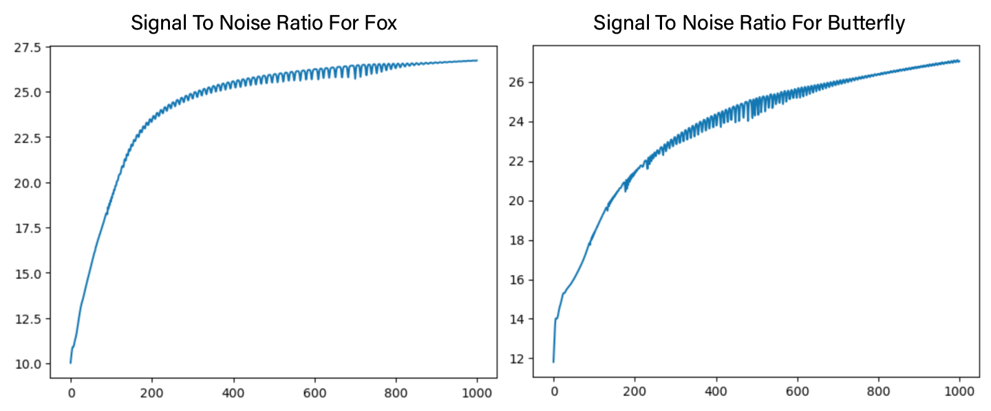
Figure 3: PSNR plot for fox and butterfly during training.
We further tested tuning the hyperparameters. Specifically, we increased the number of MLP layers by 2 and raised the positional encoding dimension to $L = 15$. The results are shown below.

Figure 4: Output image of tuned neural field at different training step.
There doesn’t seem to be any perceptible difference between the tuned version and the original. However, if we examine the PSNR plot during training, we can see that the butterfly image converged to a higher PSNR ratio, despite having a noisier trajectory.
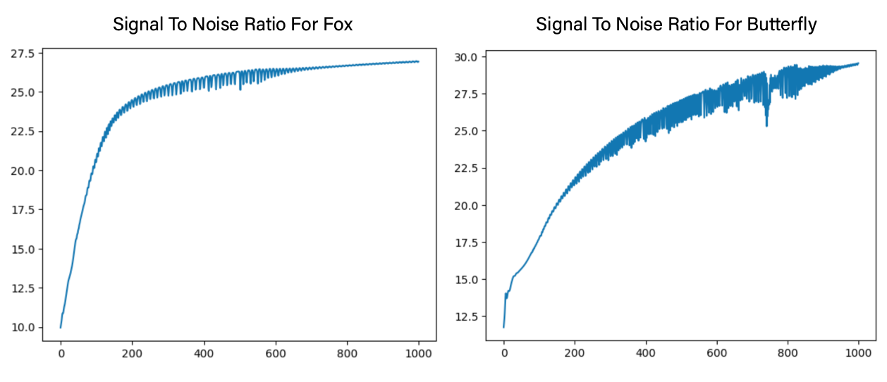
Figure 5: PSNR plot for fox and butterfly of tuned model during training.
Part B: Neural Radiance Fields
Dataset preparation
We now implement the neural radiance field from multiview images. We used the Lego scene from the original NeRF paper with lower resolution $200 \times 200$. For the dataset, we implemented the following helper functions:
transform(c2w, x_c): Transforms a point from camera coordinates to world coordinates.
pixel_to_camera(K, uv, s): Transforms a point from pixel coordinates to camera coordinates.
pixel_to_ray(K, c2w, uv): Takes in a pixel coordinate and returns the ray origin and ray direction. This is done by
We then implemented a RayDataset class. The sampling method involves the following steps:
- From the training image, sample $n_{\text{image}}$ samples.
- For each sampled image, sample $n_{\text{points}}$ pixel coordinates.
- Retrieve the RGB color at those points.
- Compute the ray origin and ray direction using the
pixel_to_rayfunction, retrieving the corresponding camera intrinsic. - Return the ray origin, ray direction, and RGB color, each of shape $(N, 3)$, where $N$ is the total number of points sampled.
Once we are done with the sampling, we also need to sample equally spaced points with perturbation along the sampled ray. This is done by sampling points on $\mathbf{r}_o + t \mathbf{r}_d$, where $t$ are the values sampled from the interval $[2.0, 6.0]$ in our implementation. We also add slight noise to $t$ during training to prevent overfitting. The sampled rays are shown below.
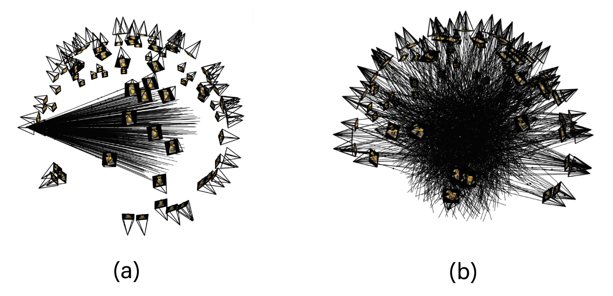
Figure 6: Example of sampled rays and points from (a) one image (b) multiple images.
NeRF Implemnetation
The NeRF model is again parameterized by an MLP. The model takes in the 3D coordinate $x$ and ray direction $d$, and outputs the density and RGB values. We follow the architecture as shown in the figure.

Figure 7: NeRF architecture.
We applied separate positional encoding on the $x$ and $d$, with $L_x$ and $L_d$ set to $10$ and $4$, respectively. The color rendered is given by the discrete approximation of the volume rendering equation:
\[\hat{C}(\mathbf{r}) = \sum_{i=1}^N T_i(1 - \exp(-\sigma_i \delta_i)) \mathbf{c}_i \hspace{5mm} \text{where} \; T_i = \exp\left(-\sum_{j=1}^{i-1} \sigma_j \delta_j \right)\]Once the rendered color is computed, the loss is the MSE loss as before. We trained the model for $2000$ epochs with the Adam optimizer and a learning rate of $5 \cdot 10^{-4}$. We sampled $100$ images, and for each image, $100$ rays were sampled. The rendered results during training are shown below.

Figure 8: Rendered results during training.
The PSNR of the training and validation set is plotted below.
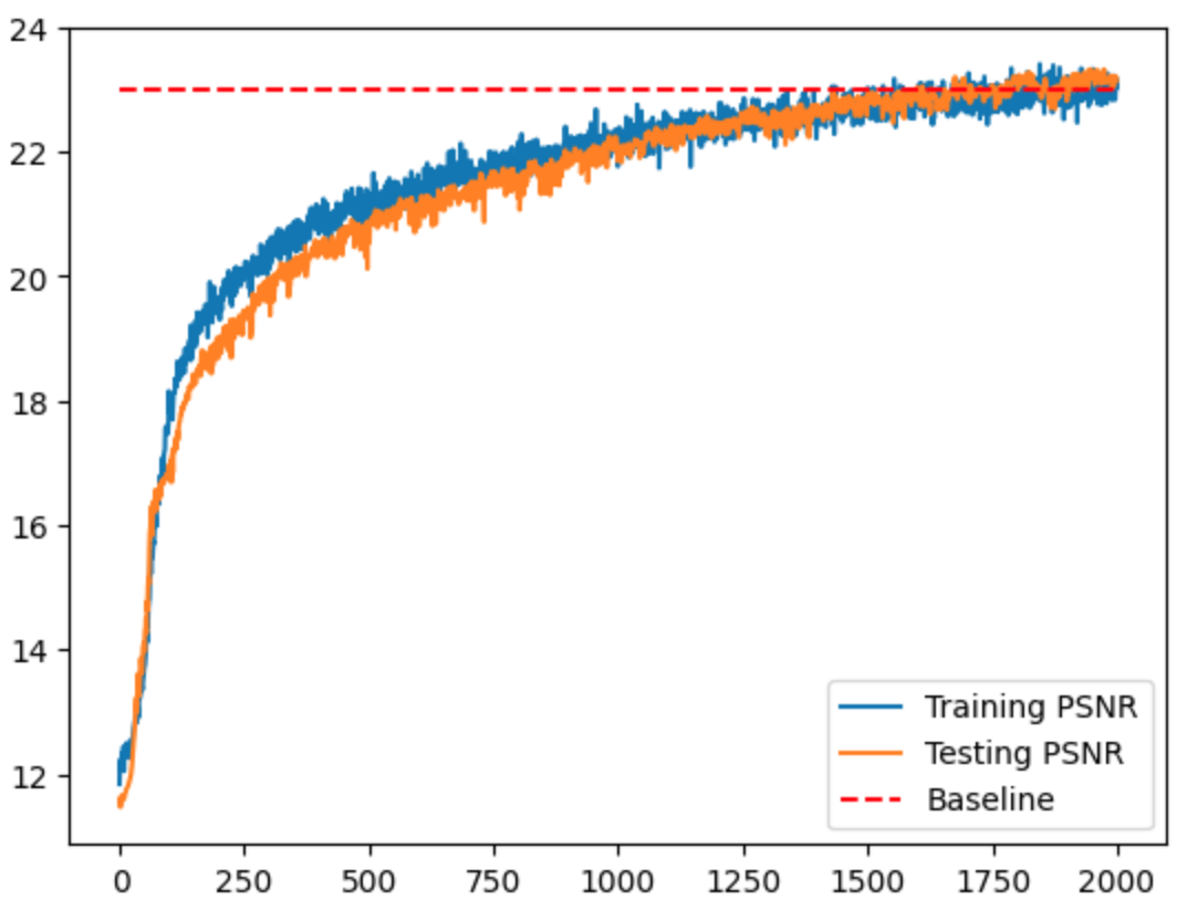
Figure 9: Training and validation PSNR curve.
Once we trained the model, we can generate novel view images of the Lego scene from arbitrary camera extrinsics. Below is a spherical rendering of the Lego scene using the provided camera extrinsics.
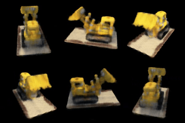
Figure 9: Novel view generation.
Bells and Whistle
For the Bell and Whistle, we in addition rendered the depth map. Instead of compositing per-point colors in volume rendering, we composite per-point depths to the pixel depth. The result, however, seems a but blurry at the bottom. One reason could be that the model is not trained enough or undersampling during training.
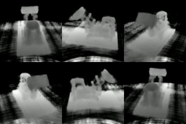
Figure 10: Rendered depth map.