Project 5

Part A: The Power of Diffusion Models!

A.1 Forward Process

Before diving into diffusion models, we first focus on the problem of denoising—removing noise from noisy images. The data we will use consists of a collection of noisy images at different scales. The noisy image is defined as:

\[x_{noised} = x + \sigma \epsilon\]

where $x$ denote the clean image and $\epsilon \sim N(0, 1)$.

We show a few examples of noisy images at scales $250$, $500$, and $700$, respectively, in the figure below.

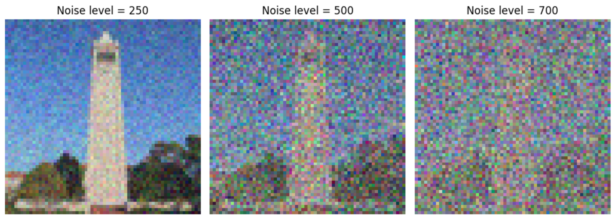
Figure 1: Noised images of different scale.

A.2 Classical Denoising

We now attempt to denoise the images. The classical approach to denoising is to apply a Gaussian filter, as shown below.

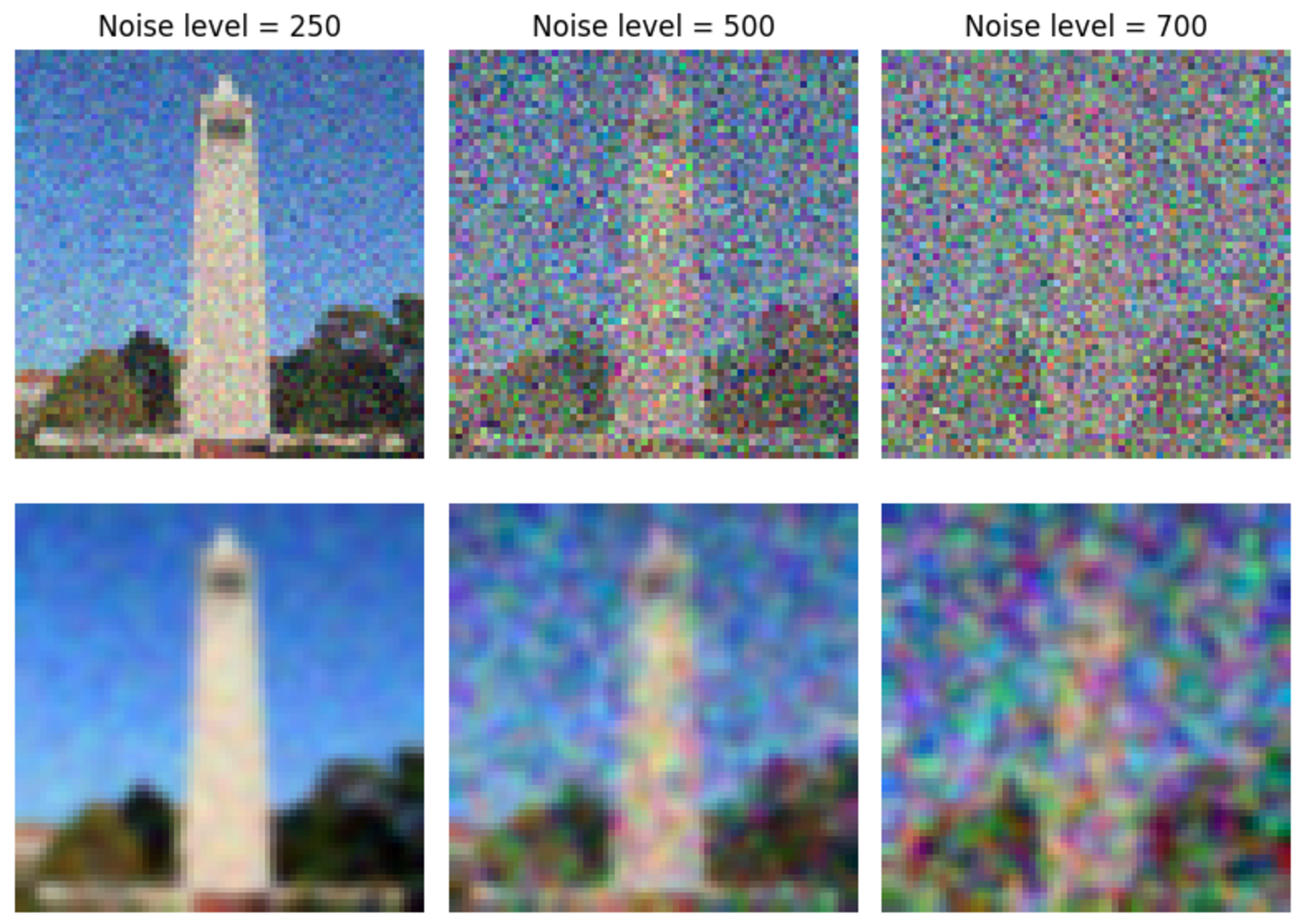
Figure 2: Gaussian denoising (Top row) Noisy image (Bottom row) Gaussian denoised images.

Note that the Gaussian filter is not sufficient to completely remove the noise.

A.3 One-Step Denoising

We now use a pretrained diffusion model for denoising. Specifically, we utilize the DeepFloyd IF diffusion model, which supports text prompts. Below, we showcase some examples of DeepFloyd IF generations along with their corresponding prompts. The seed that we are using is $180$.

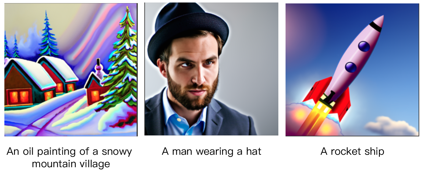
Figure 3: Sample generation of DeepFloyd model.

Note that the pretrained diffusion model is capable of generating high quality images that are related to the text prompt. Using the UNet architecture from DeepFloyd IF, we apply single-step denoising, which estimates the original image using

\[x_0\approx \frac{1}{\sqrt{\bar{\alpha_t}}}(x-\sqrt{1-\bar{\alpha_t}}\epsilon)\]

The results are presented below.

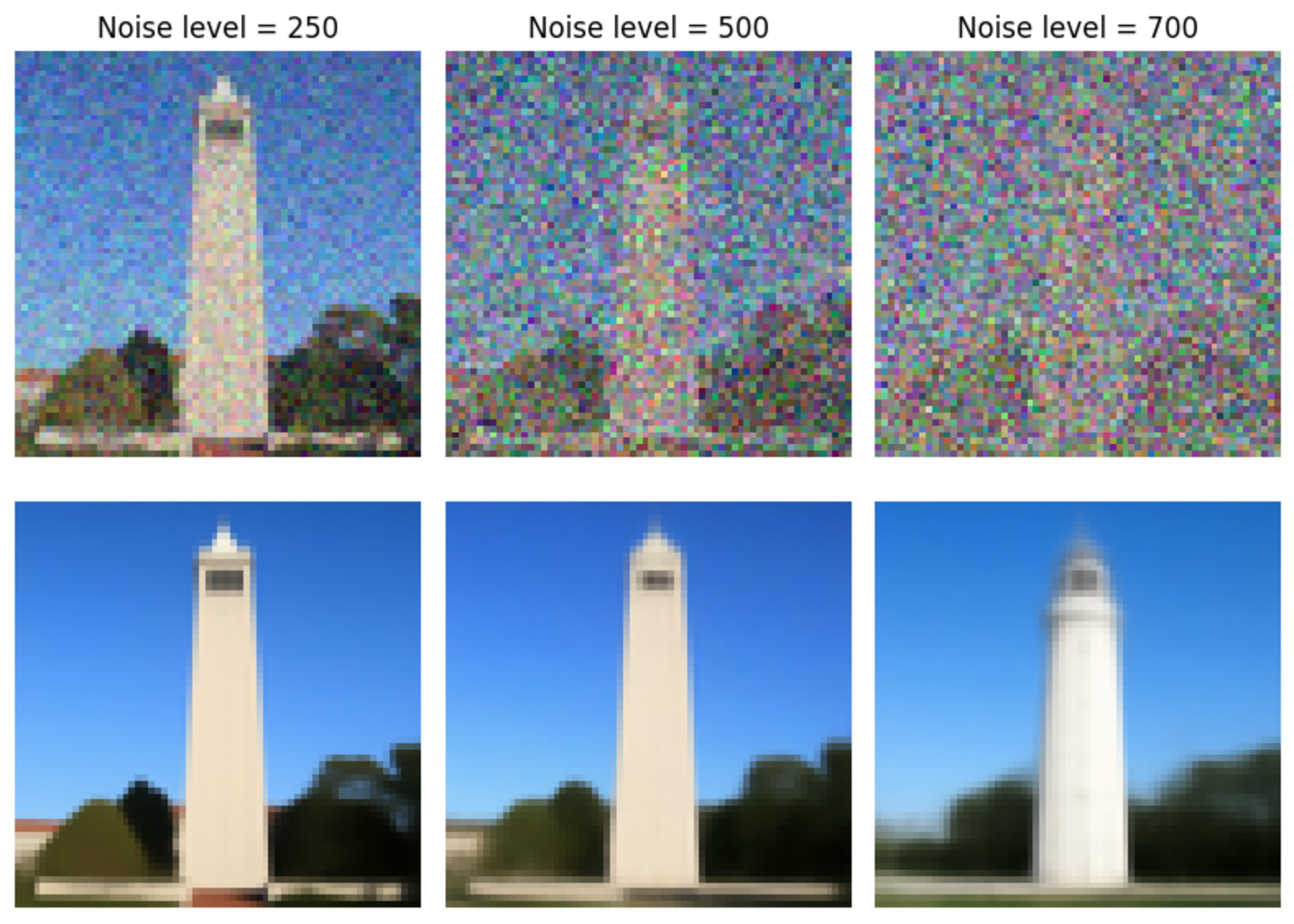
Figure 4: One step denoised images (Top) Noisy image (Bottom) One-step denoised image. For the original image, see Figure 6.

Note that the denoised results are significantly better compared to Gaussian denoising.

A.4 Iterative Denoising

To further improve the performance of denoising, we can increase the number of steps, leading to an iterative denoising method. Once we estimated $x_0$, we then update $x_t$ to a less noisy image $x_{t’}$ using

\[x_{t'} = \frac{\sqrt{\bar{\alpha_{t'}}}\beta_t}{1-\bar{\alpha_t}}x_0+\frac{\sqrt{\alpha_t}(1-\bar{\alpha_{t'}})}{1-\bar{\alpha_t}}x_t+v_\sigma\]

To simplify the calculations, we used strided timesteps. The noised images are shown below.

Figure 5: Noisy images.

Comparing the results of iterative denoising with other methods, we observe that iterative denoising provides the best results with the finest details.

Figure 6: Comparison of different methods.

A.5 Diffusion Model Sampling

In the previous section, we used the diffusion model for denoising. However, we can also use the iterative denoising method to generate images. By starting with a random image and progressively denoising, we can achieve the desired results. Some examples are shown below, using the prompt set to "a high-quality photo."

Figure 7: Sample generated images using the diffusion model.

A.6 Classifier-Free Guidance (CFG)

We can enhance the quality of the images through classifier-free guidance, which uses both conditional and unconditional noise estimates to represent the noise. The noise $\epsilon$ is given by

\[\epsilon = \epsilon_u + \gamma(\epsilon_c - \epsilon_u)\]

where $\gamma$ is a parameter that controls the strength of guidance. Below are some examples of images generated using classifier-free guidance.

Figure 8: Sample generated images using classifier free guidance.

A.7 Image-to-image Translation

SDE Edit

We now move on to different applications of image generation. The first application is image editing, which involves slightly noising the image and then performing denoising using the iterative denoiser from A4. Below are the results of applying different noise levels to the test image.

Figure 9: SDEdit on test image.

Note that the images gradually resemble the original images. We can also apply the same method to images of our choice, including web images and hand-drawn images.

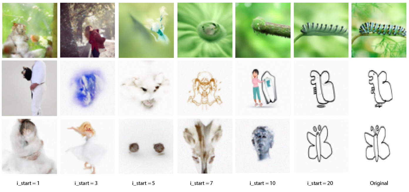
Figure 10: More SDEdit examples.

Inpainting

Another similar application is inpainting. By removing certain regions of an image and filling them with noise, we can generate new parts for the image. Below are some examples using the test image and a few internet images.

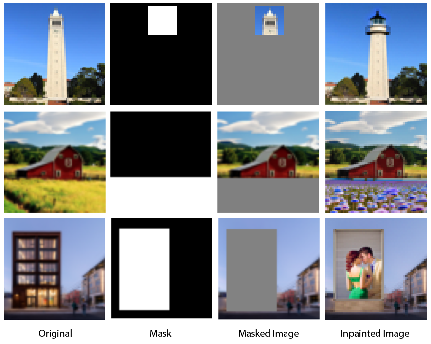
Figure 11: Inpainting image examples.

Text-Conditional Image-to-Image Translation

During the process of reverse diffusion, we can also guide the process using different prompts. Below are some examples with different prompts. The prompts for the three rows are "a rocket ship", "a pencil", and "a photo of a dog", respectively.

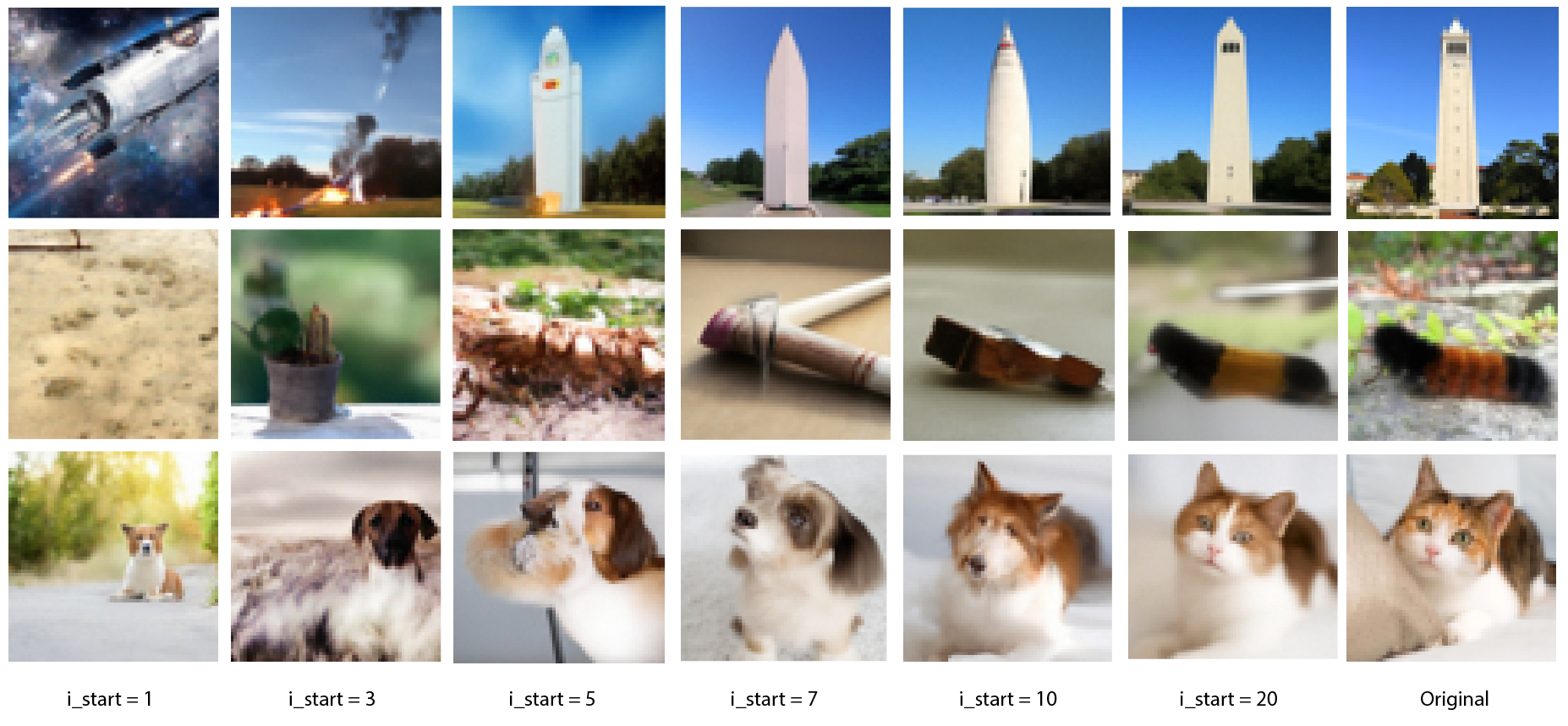
Figure 12: Text conditional generation examples.

A.8 Visual Anagrams

Diffusion models can also be used to create optical illusions. We allowed the approach of Visual Anagrams: Generating Multi-View Optical Illusions with Diffusion Models to generate anagrams. The idea is that we input two prompts, which is used to make two different noise estimates

\[\epsilon_1=\epsilon_\theta(x_t, t, p_1)\hspace{5mm}\epsilon_2=\text{flip}(\epsilon_\theta(\text{flip}(x_t), t, p_2))\]

The final noise estimate will then become the average of these two. Below shows some reuslt of visual anagrams.

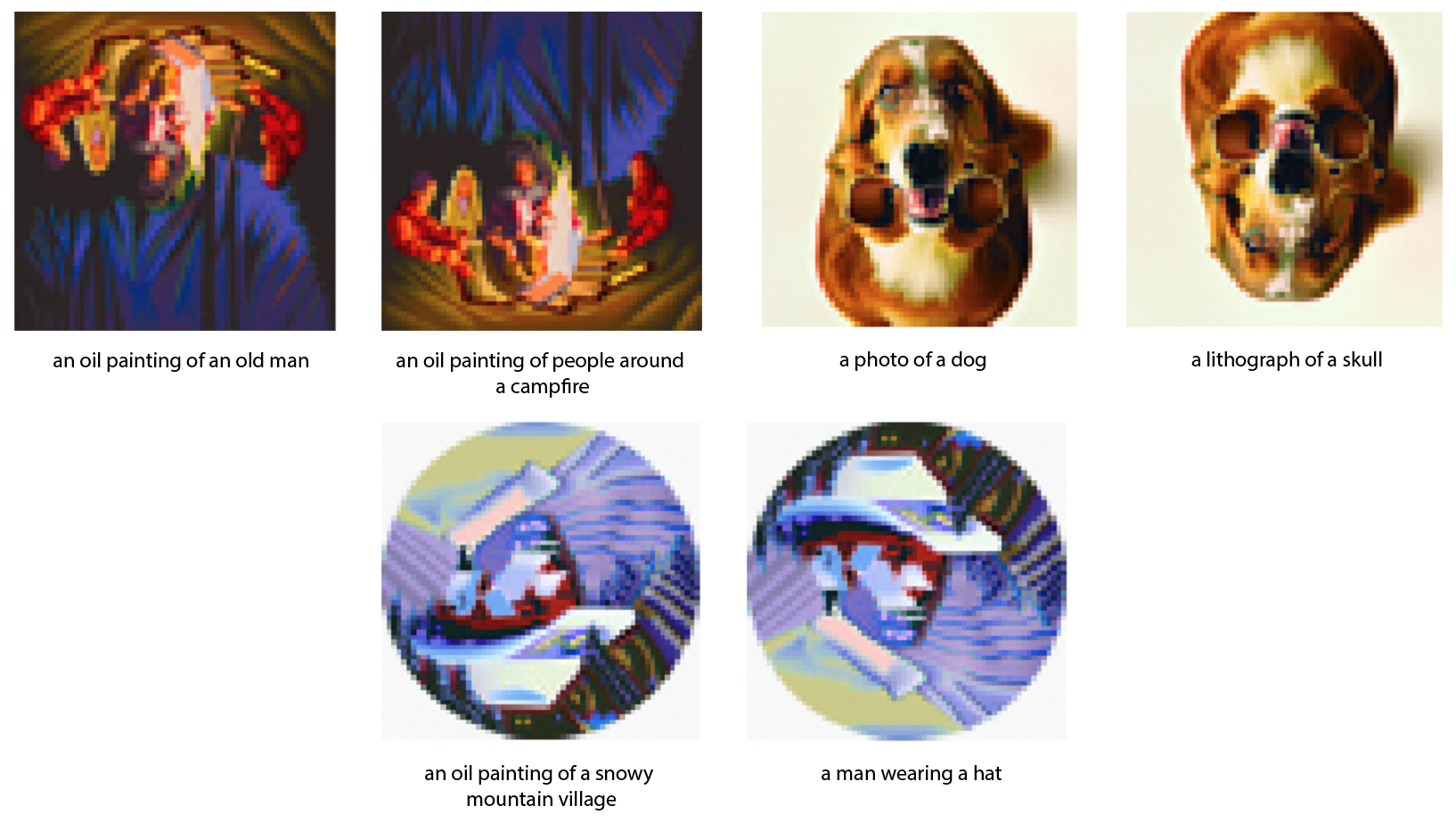
Figure 13: Generated visual anagrams.

A.9 Hybrid Images

We can also create hybrid images. Similar to before, we take in two prompts, $p_1$ and $p_2$. The noise estimates for the prompts are:

\[\epsilon_1 = \epsilon_\theta(x_t, t, p_1) \hspace{5mm} \epsilon_2 = \epsilon_\theta(x_t, t, p_2)\]

The final noise estimate is then given by:

\[\epsilon = f_{low \, pass}(\epsilon_1) + f_{high \, pass}(\epsilon_2)\]

The rest of the process follows the same procedure. Some examples of generated hybrid images are shown below.

Figure 14: Generated hybrid images.

Part B: Diffusion Models

Denoiser Model

We will now implement a diffusion model from scratch. Before implementing the diffusion model, we begin by implementing a denoiser, which takes in a noised image and tries to remove the noise present. To do this, we use the U-Net architecture as suggested in the project description. The dataset is MNIST, which has been corrupted with additive noise, as follows:

\[z_i=x_i+\sigma \epsilon_i\]

We show the impact of different noise in the figure below.

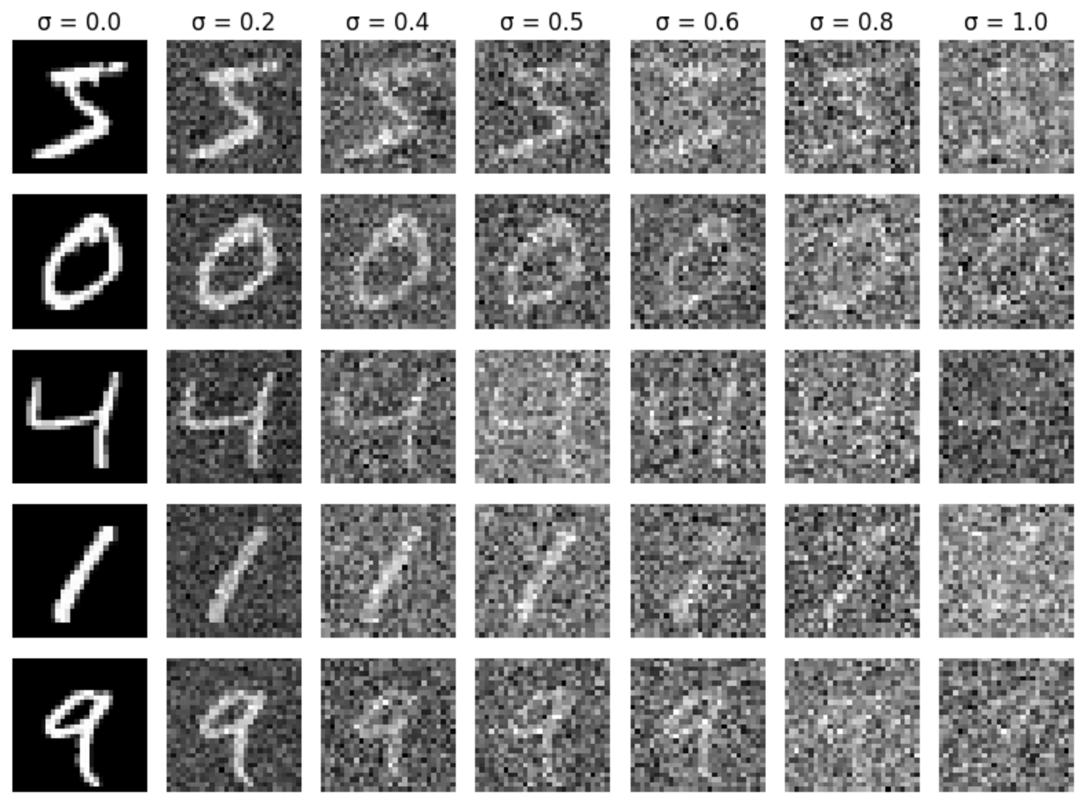
Figure 15: MNIST with different noise level.

The network, during training, takes in a noised image and tries to output the desnoised image, the stochastic loss is then defined by

\[L =\frac{1}{n}\sum_{i=1}^n ||D_{\theta}(x_i+\sigma\epsilon_i) - x_i||_2^2\]

For the purpose of our training, we set $\sigma=0.5$. The network is trained for $5$ epochs with Adam optimizer with learning rate $10^{-4}$ and batch size of $32$. The training loss curve is shown below.

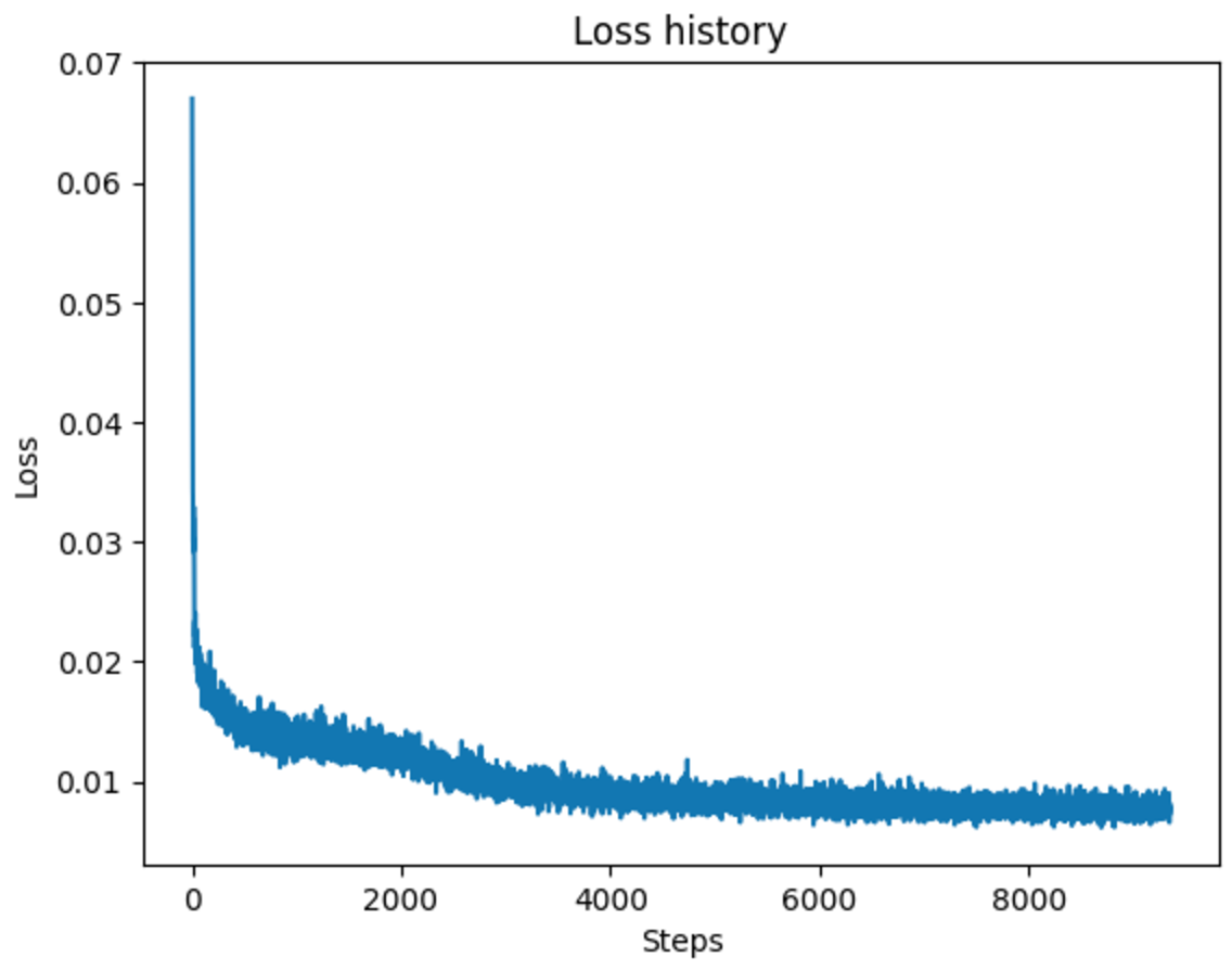
Figure 16: Training loss curve for denoiser model.

We display the denoising result after the 1st and 5th epochs as below.

Figure 17: Sample denoised results after 1st epoch. (Top row) Original image (Middle row) Corrupted image (Bottom row) Denoised image

We can see that the model has already learned how to denoise the corrupted images. Extending the training to 5 epochs gives us better results.

Figure 18: Sample denoised results after 5th epoch. (Top row) Original image (Middle row) Corrupted image (Bottom row) Denoised image

We see that the model successfully removed the noises and recovered the handwritten images. We can also test the models’ performance on different noise level. From the figure below, we can see that our model is quite robust at different noise levels, despite not being trained on them.

Figure 18: Denoiser is able to denoise images of different noise levels.

Diffusion Model

We now train a diffusion model. To do so, we first slightly modify the architecture of the U-Net to allow conditioning on the timestep. This is achieved through two linear layers with GeLU activation. The training of a diffusion model works as follows: at each step, we sample a timestep $p$, then noise the image according to:

\[x_t = \sqrt{\bar{\alpha_t}}x_0 + \sqrt{1-\bar{\alpha_t}}\epsilon\]

where $\epsilon$ is sampled from a normal distribution. The model $\epsilon_{\theta}$ then tries to recover the noise that has been added. The final loss is the MSE between the estimated noise and the true noise. We trained the model for 20 epochs with an exponential scheduler and the Adam optimizer with a learning rate of $10^{-3}$. The training loss is shown below.

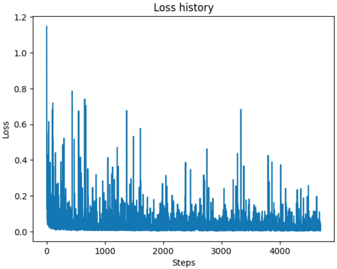
Figure 19: Diffusion model training loss curve.

We generated samples during training. Some results are shown below. That that the model is capable of generating digits that is similar to the training data.

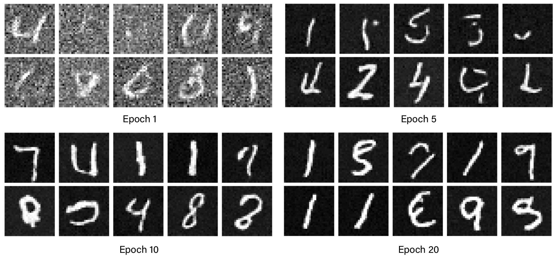
Figure 20: Sample generation at different stage of training.

Diffusion Model With Class Conditioning

Note that the samples generated from the diffusion model can be any digit. We can add control by incorporating class conditioning, which works similarly to time conditioning, except that we pass a one-hot encoded class into the linear layers. We follow the modulated approach as suggested in the project description. Additionally, we added random dropouts with $p=0.1$ so that the model is sometimes trained without labels. Training the class-conditioned model works similarly to the previous setup. We use the same training configuration, and the training loss curve is shown below.

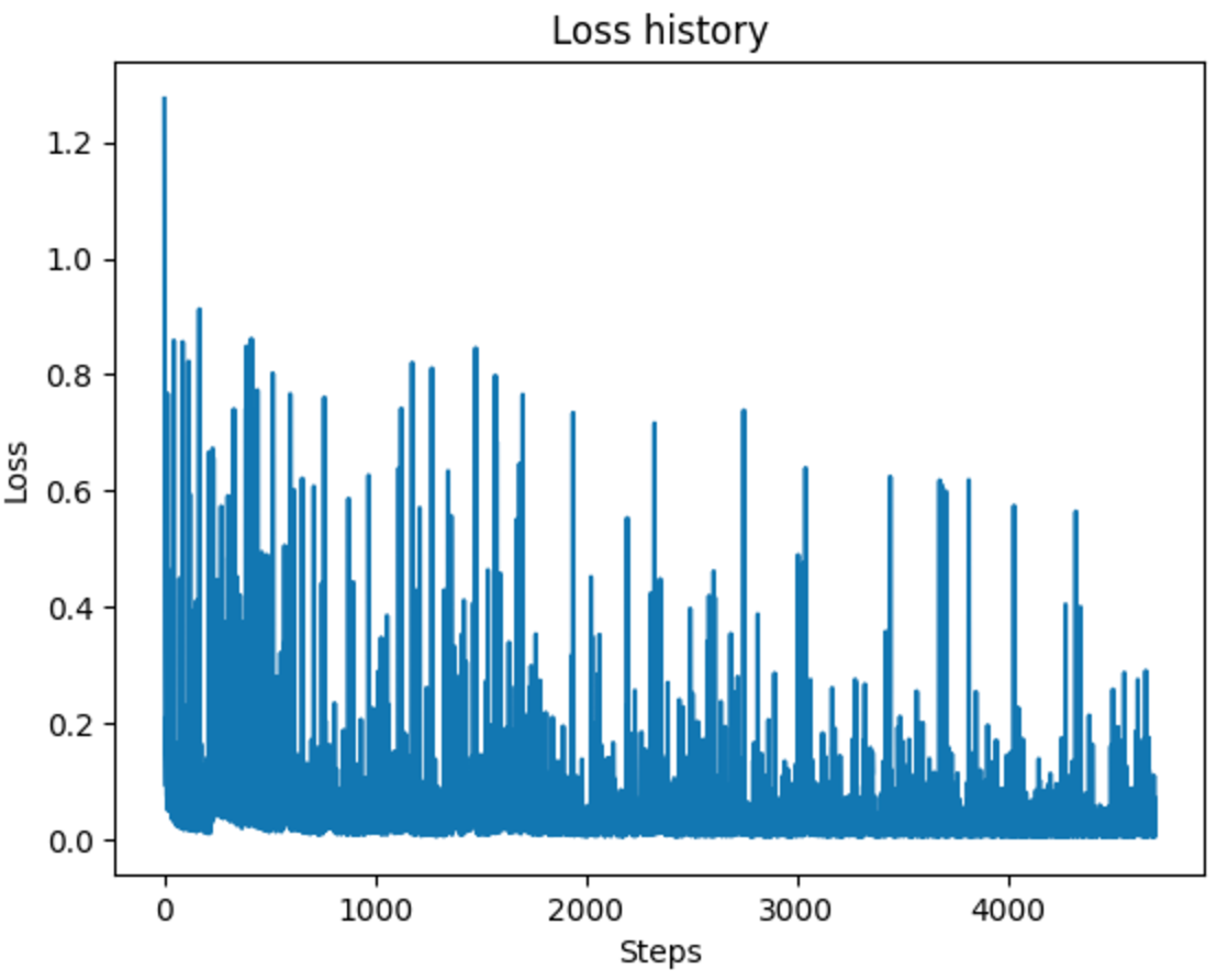
Figure 21: Training loss of class-conditioned diffusion model.

Like before, we generated samples during training. Note that now the model is capable of generating the specific digits we specify.

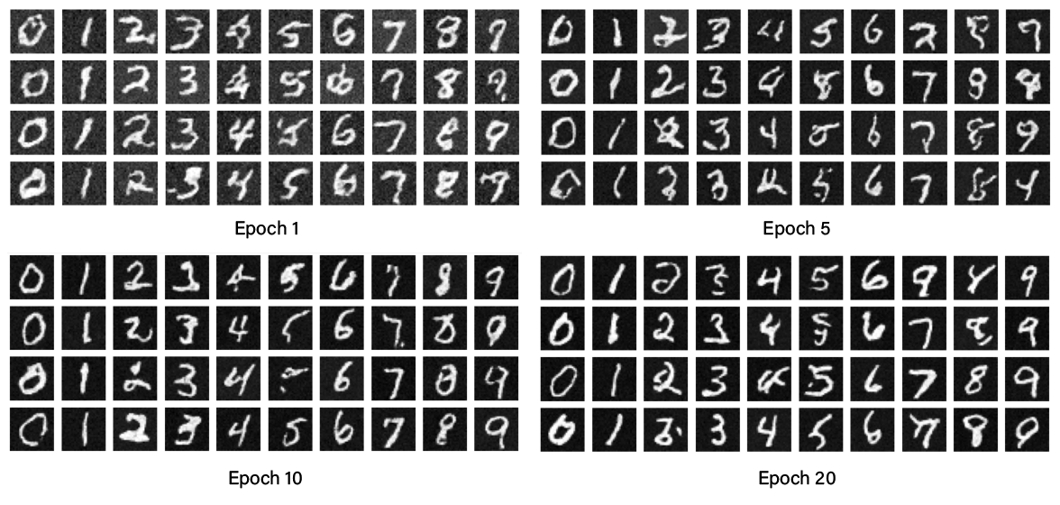
Figure 1: Labeled source and target images.