Project 4

Image Warping and Mosaicing

Image Labeling

The goal of this project is take two images in different angles and create an image mosaic by aligning, warping, and compositing them. We first take images of our choices and uses online labeling tool to label eight correspondence points. We will be using these points to estimate a homography map for registration later.

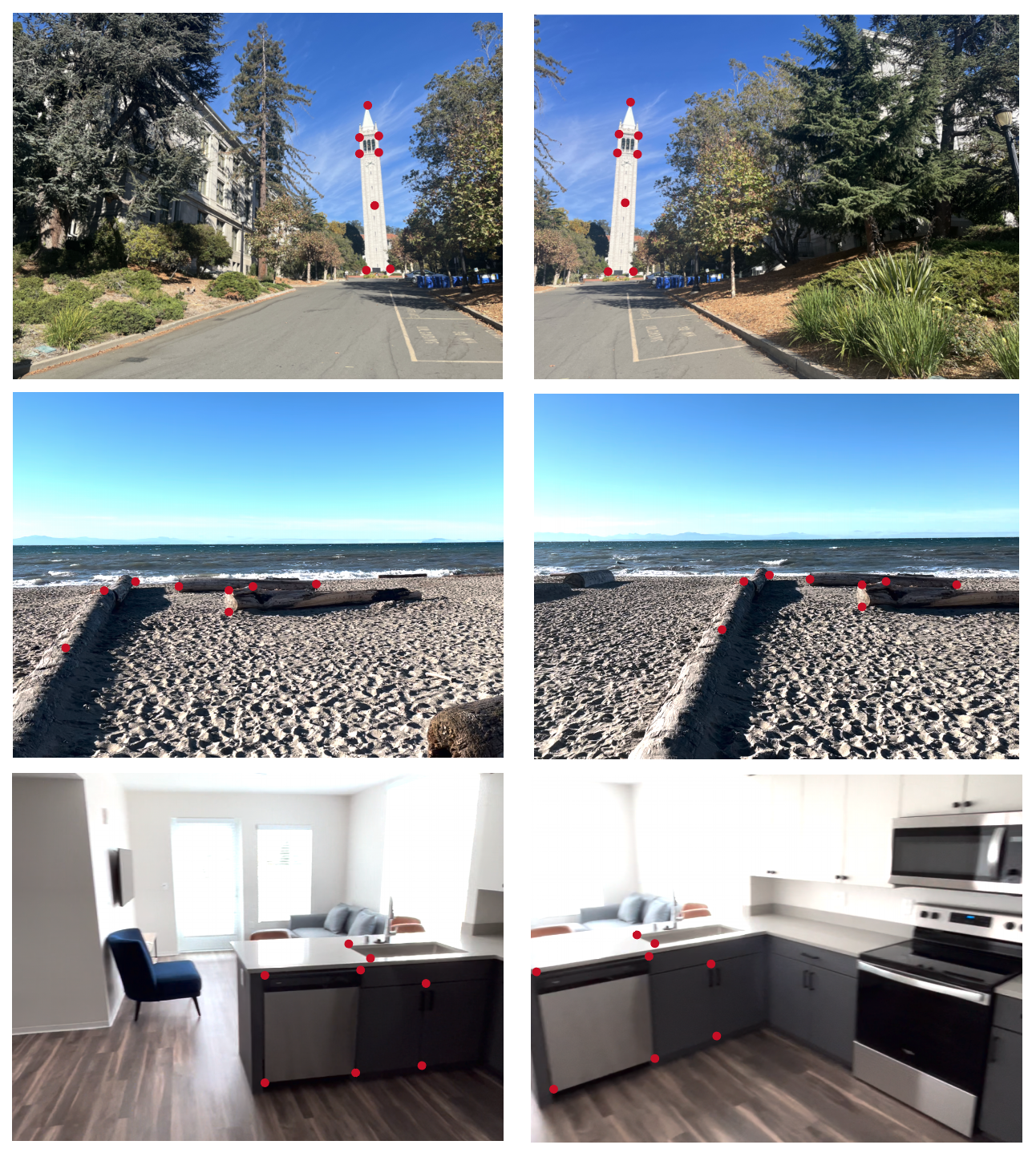
Figure 1: Labeled source and target images.

Homography Estimation and Warping

Given a list of source points $\mathcal{S}= {(x_i, y_i)}$ and target points $\mathcal{T}={(\tilde{x}_i, \tilde{y}_i)}$, to estimate a homography matrix $\mathbf{H}$, note that each source-target pair imposes the constraint

\[\begin{bmatrix} a & b & c\\ d & e & f\\ g & h & 1 \end{bmatrix}\begin{bmatrix} x_i\\ y_i\\ 1 \end{bmatrix}=\begin{bmatrix} \xi \tilde{x}_i\\ \xi \tilde{y}_i\\ \xi \end{bmatrix}\]

Simplifying gives us

\[\begin{bmatrix} x_i & y_i & 1 & 0 & 0 & 0 & -x_i\tilde{x}_i & -y_i\tilde{x}_i\\ 0 & 0 & 0 & x_i & y_i & 1 & -x_i\tilde{y}_i & -y_i\tilde{x}_i\\ \end{bmatrix} \begin{bmatrix} a\\ b\\ c\\ d\\ e\\ f\\ g\\ h\\ \end{bmatrix} =\begin{bmatrix} \tilde{x}_i\\ \tilde{y}_i \end{bmatrix}\]

Since there are $8$ variables, $4$ correspondence points are needed to estimate a unique homography transformation. However, one can also choose more than $4$ points and then solve the system using least squares. In our case, we choose $8$ correspondence points for each image and estimated the homography transformation using the np.lstsq function. After estimating the homography matrix, we can then apply inverse warp as in the previous project.

Aside: Image Rectification

To test our approach, we can attempt to warp objects in an image into a square. This is done by specifying four correspondence points and mapping them to a rectangle. Below are some of the rectification results.

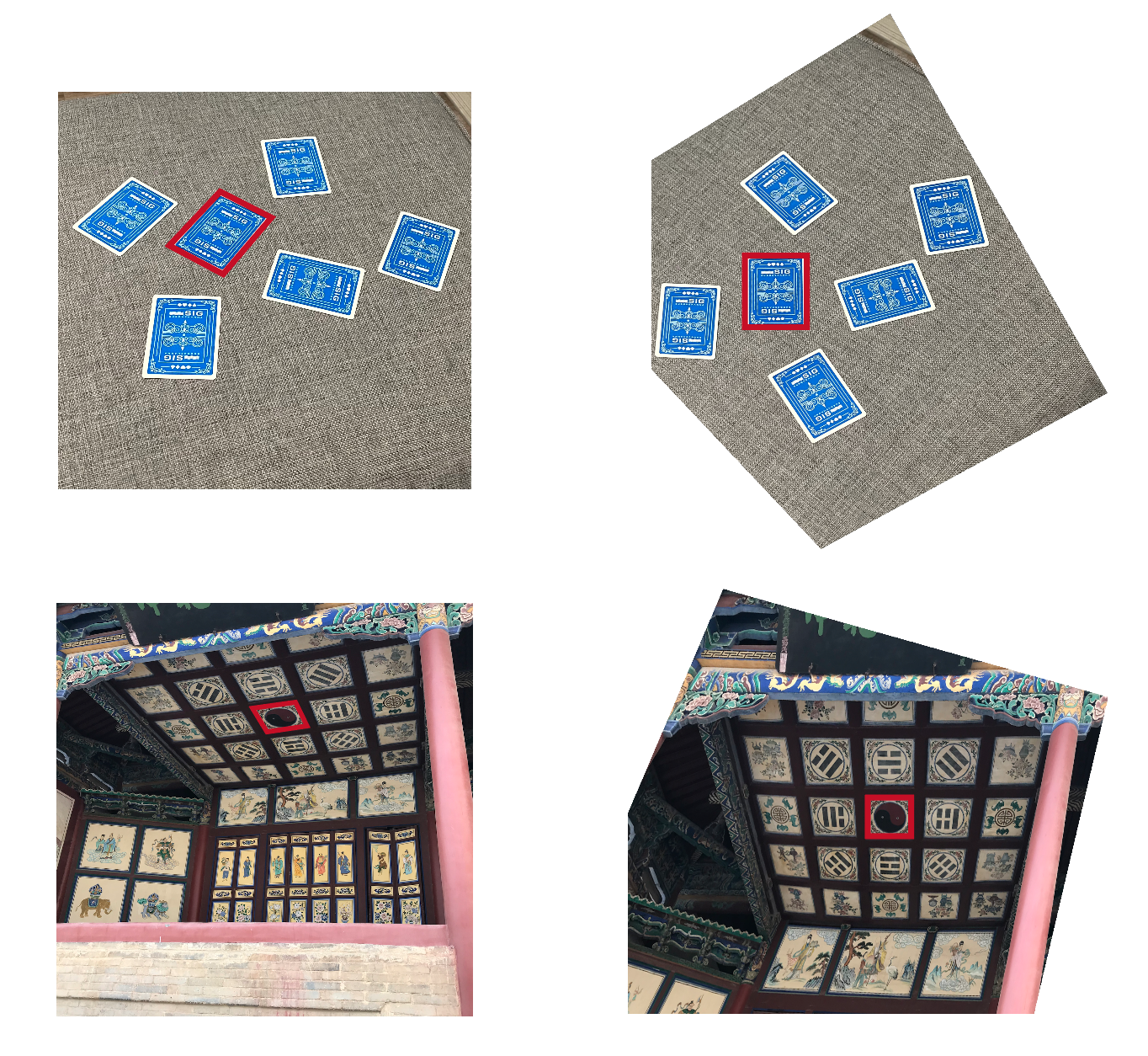
Figure 2: Rectified image. The second image in cropped for view.

Image Mosaic

We warped the target images with the estimated homography transformation, this gives us the following. Note that the images are now aligned.

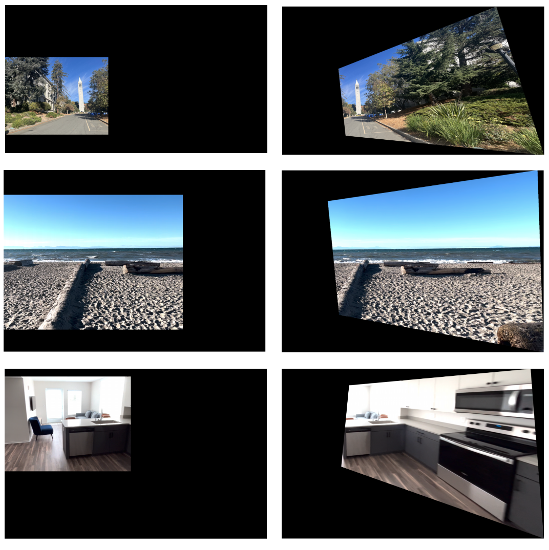
Figure 3: Warped and aligned source/target images.

We now blend the image using the Laplacian pyramid approach with vertical binary masks. Below shows the final results of the image mosaic.

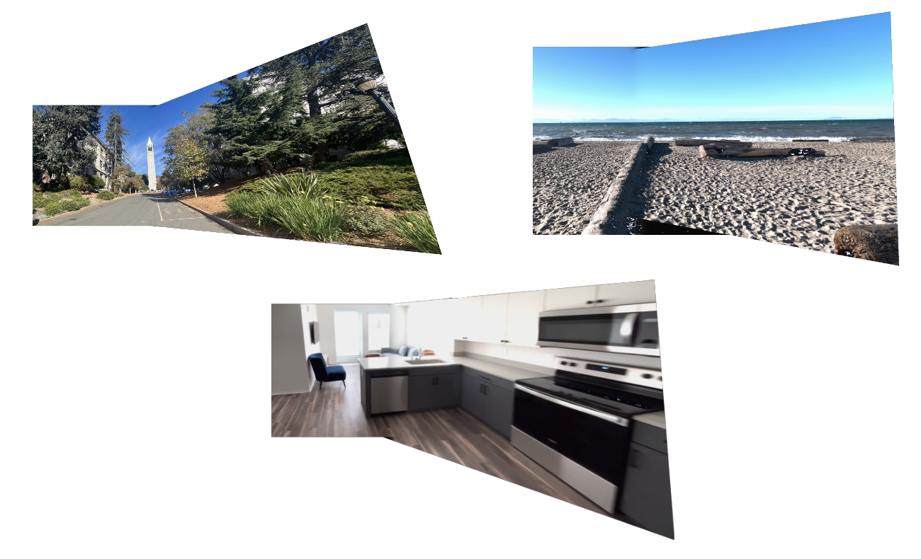
Figure 4: Mosaic images.

Automatic Image Warping and Mosaicing

In the previous section, we manually labeled keypoints for both images. In this section, we will automatically detect “interesting” keypoints in an image and perform warping. The steps include:

1. Keypoint detection
2. Adaptive non-maximum suppression
3. Feature matching
4. Robust homography estimation

Keypoint detection

To find the keypoints, we used the Harris corner detector. The idea is that corners in an image exhibit a strong signal in all directions when the local patch is shifted slightly by $(\Delta x, \Delta y)$.

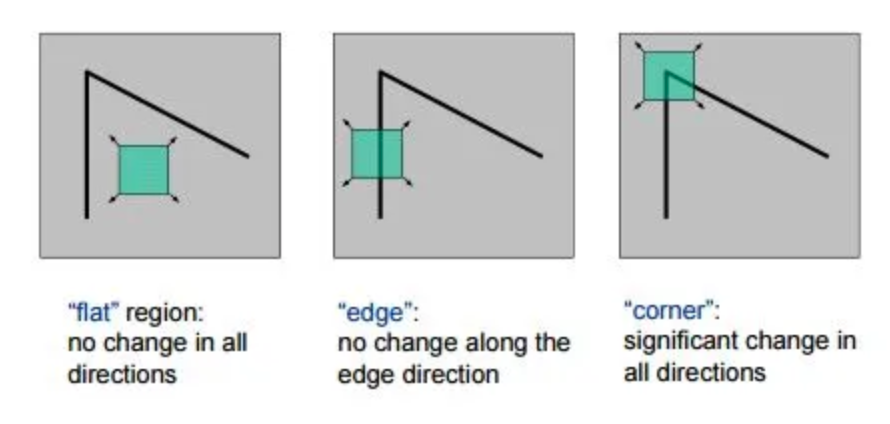
Figure 5: Harris corner detection.

The shifted patch can be estimated using a Taylor expansion.

\[\begin{equation*} \begin{aligned} E(\Delta x, \Delta y) &= \sum_{(\Delta x, \Delta y)} (I(x+\Delta x, y+\Delta y)-I(x, y))^2 \\ &\approx \sum_{(\Delta x, \Delta y)} (I_x \Delta x + I_y \Delta y)^2\\ &= \begin{bmatrix}\Delta x & \Delta y\end{bmatrix}\bigg(\sum_{(\Delta x, \Delta y)} \begin{bmatrix}I_x^2 & I_xI_y\\ I_yI_x & I_y^2 \end{bmatrix}\bigg)\begin{bmatrix}\Delta x \\ \Delta y\end{bmatrix} \end{aligned} \end{equation*}\]

Let ( M ) denote the matrix in the middle. The score, or the measure of corner response at each position, is then computed by

\[R = \text{det}(M) - k \, \text{Tr}(M)\]

where ( k ) is a sensitivity parameter. We can then filter out weak corners by setting a threshold. Examples of detected corners are shown below.

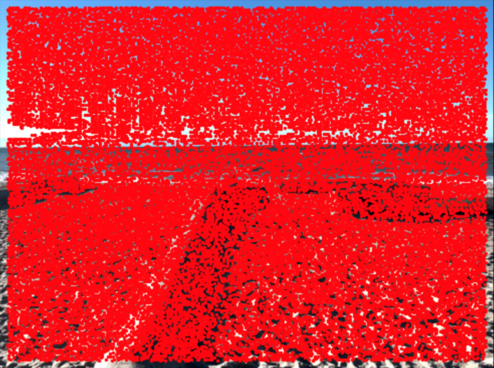
Figure 6: Harris corner detection of beach image.

Adaptive Non-Maximum Suppression

The Harris corner detector detects many corners. If we proceed directly to feature matching, it would be time-consuming. To address this, we first adaptively filter out corners with weak responses, following the approach from Brown et al. Specifically, we compute the suppression radius $r_i$ for each interest point $\mathbf{x}_i$, defined as

\[r_i = \min_j ||\mathbf{x}_i - \mathbf{x}_j||_2^2\;\;\;\;\;\;\;\;\;\;R(\mathbf{x}_j) < c_{robust}R(\mathbf{x}_j)\]

Here, ( c_{\text{robust}} ) is a hyperparameter set to ( 0.9 ) in this work. After computing the suppression radius (which can be optimized using a K-d tree for better runtime), we select the interest points with the highest suppression radius values. This ensures that the keypoints are evenly distributed across the image.

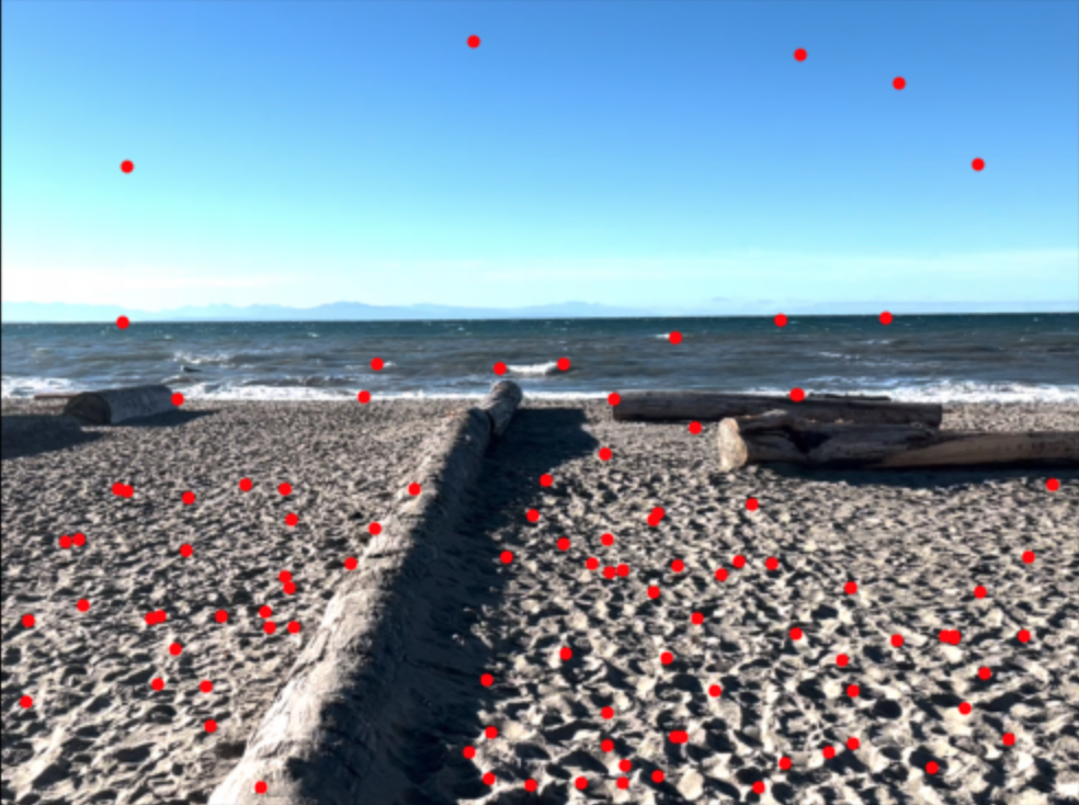
Figure 7: Adpative non-maximum suppression.

Feature Matching

We now proceed to feature matching. To match features, we sample a $40 \times 40$ patch around each keypoint and downsample it to an $8 \times 8$ patch. This patch is then flattened to form a feature vector, giving us two sets of feature vectors for the images, $\mathcal{S}$ and $\mathcal{T}$. To match $s_i \in \mathcal{S}$, we find its two nearest neighbors in $\mathcal{T}$ and compute the ratio of their distances. We set the match to the nearest neighbor if the ratio is sufficiently large.

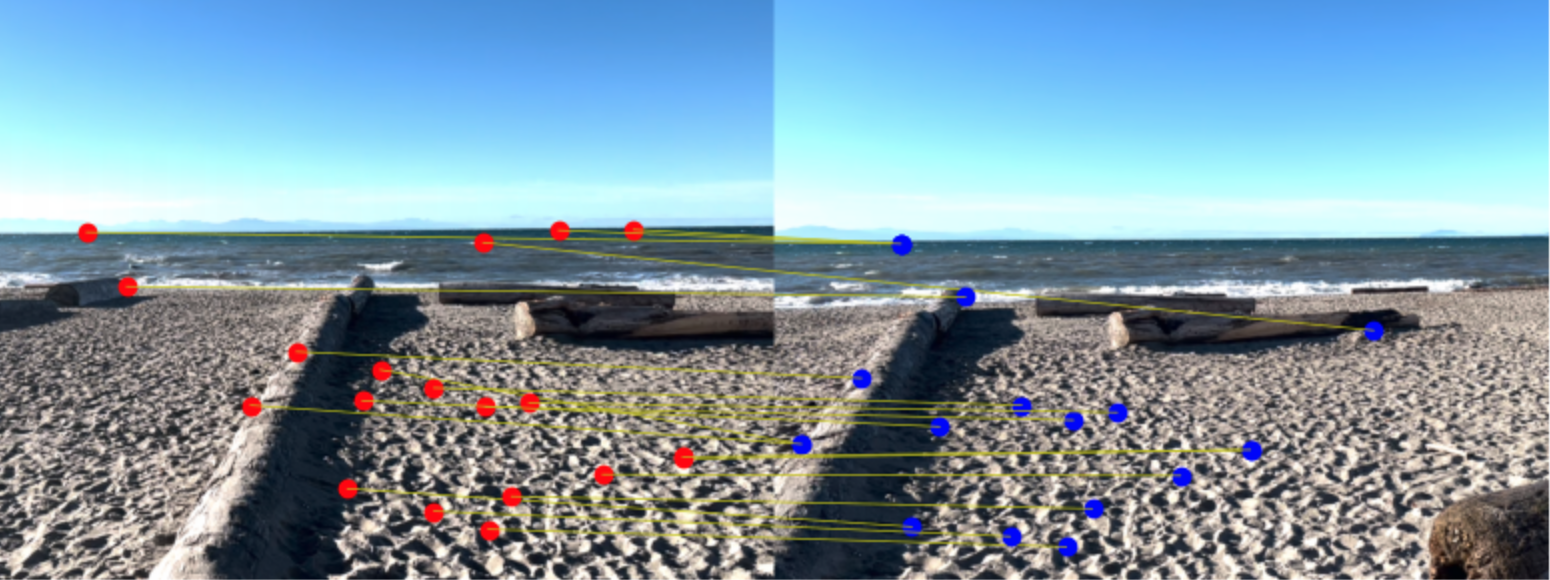
Figure 8: Matched features using Lowe's trick.

Homography estimation

The matched features from the previous step are not perfect and sometimes include outliers. To address this, we applied RANSAC homography estimation. This process involves iteratively selecting a random sample of points, fitting a homography, and calculating the number of points that “match” the homography. Throughout the iterations, we retain the homography with the highest match rate. The RANSAC results are shown below.

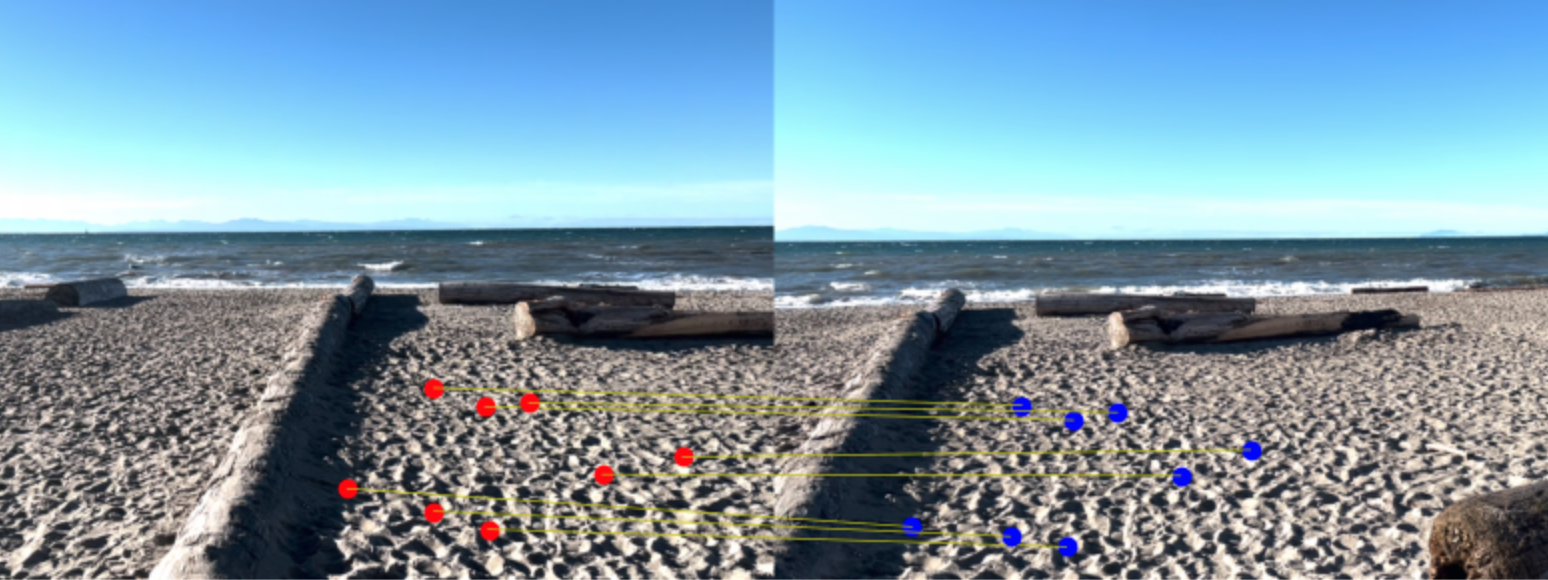
Figure 9: Ransac for robust homography estimation.

Final results

After finding the homography, we can follow the same approach as before to produce the mosaic. The results for automatic mosaicing are shown below.

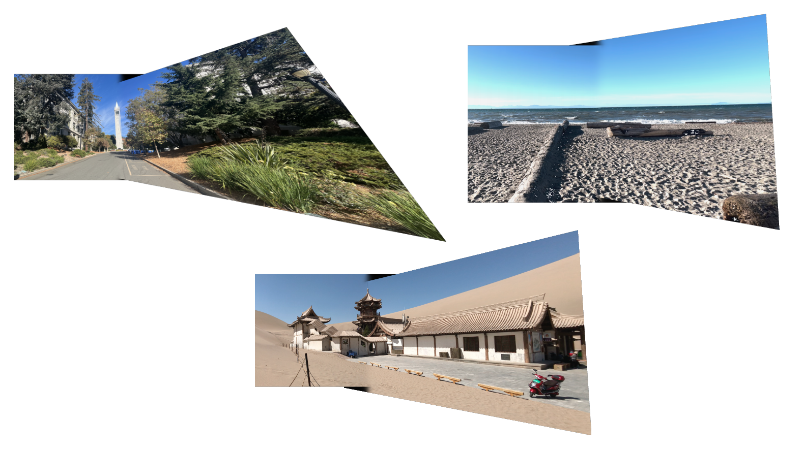
Figure 10: Automatic mosaicing.

Note that the automatic mosaicing method demonstrates good performance compared to manual labeling.

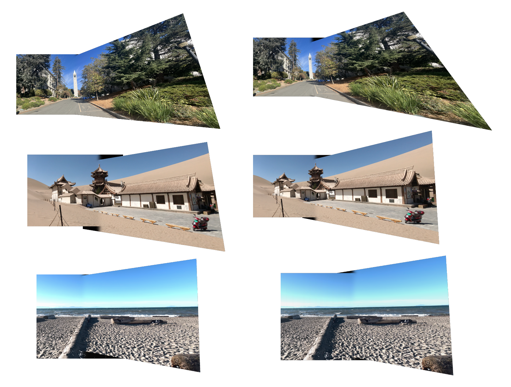
Figure 11: Comparison of manual labeling (left) and automatic labeling (right).