Project 3

Face morphing

Overview

The goal of this project is to morph two faces to create a new one. A naive approach is to directly average the two faces, as shown in Figure 1. However, this method generally does not work well because the two images are often not aligned. To morph two images, we need to follow two steps: alignment and color blending. We will walk through each of these steps in detail in this project.

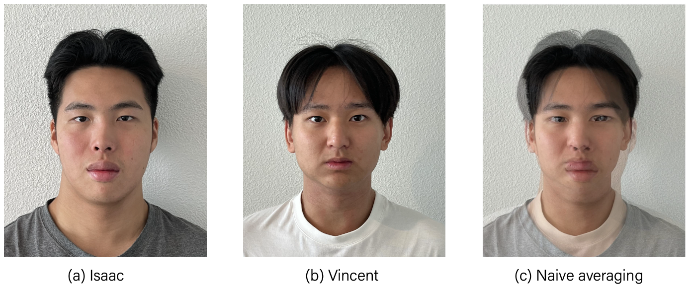
Figure 1: Blended image by taking direct average. Note that the faces are not aligned.

Morphing two faces

Defining correspondence

To align the two images, we start by labeling key points on both images. These points will serve as landmarks for the morphing process. Next, we apply Delaunay triangulation using the scipy.spatial.Delaunay library. We use the average key points to compute the triangulation, making it less dependent on the individual images. In the next section, we will map the pixel intensity values from the midway triangle to the corresponding original triangles to perform warping (Figure 2).

Figure 2: Illustration of the process: We map the triangle formed by the midway key points (b) to the corresponding triangle in the original image (a). The pixel intensity values are interpolated.

The key points for the two images and the triangulation of the midway image are shown below.

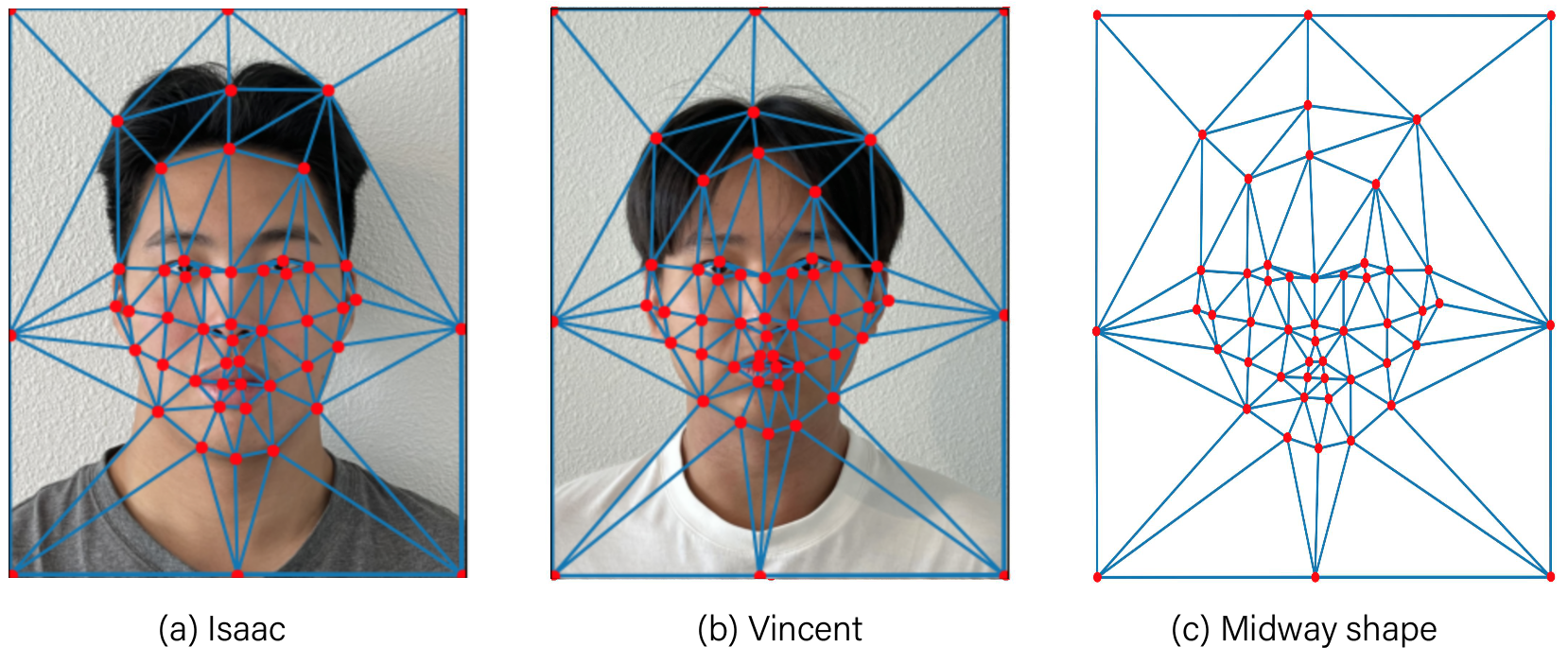
Figure 3: Triangulation of the original images (a), (b), and the midway image (c).

Computing midway face

As an initial example, we first compute the midway face of the two images. To do this, we begin by warping the images to align them. After warping, we then average the pixel values to blend the colors, resulting in the midway face.

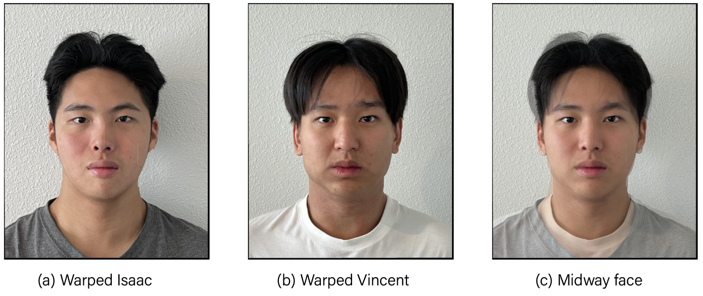
Figure 4: Midway face after alignment.

The morph sequence

We can now apply the same methods to compute the morphed image by varying the warp fraction $\alpha$ and the dissolve fraction $\beta$. The following animation is generated by changing $\alpha$ and $\beta$ in regular intervals of $0.43$ within the range $[0,1]$.

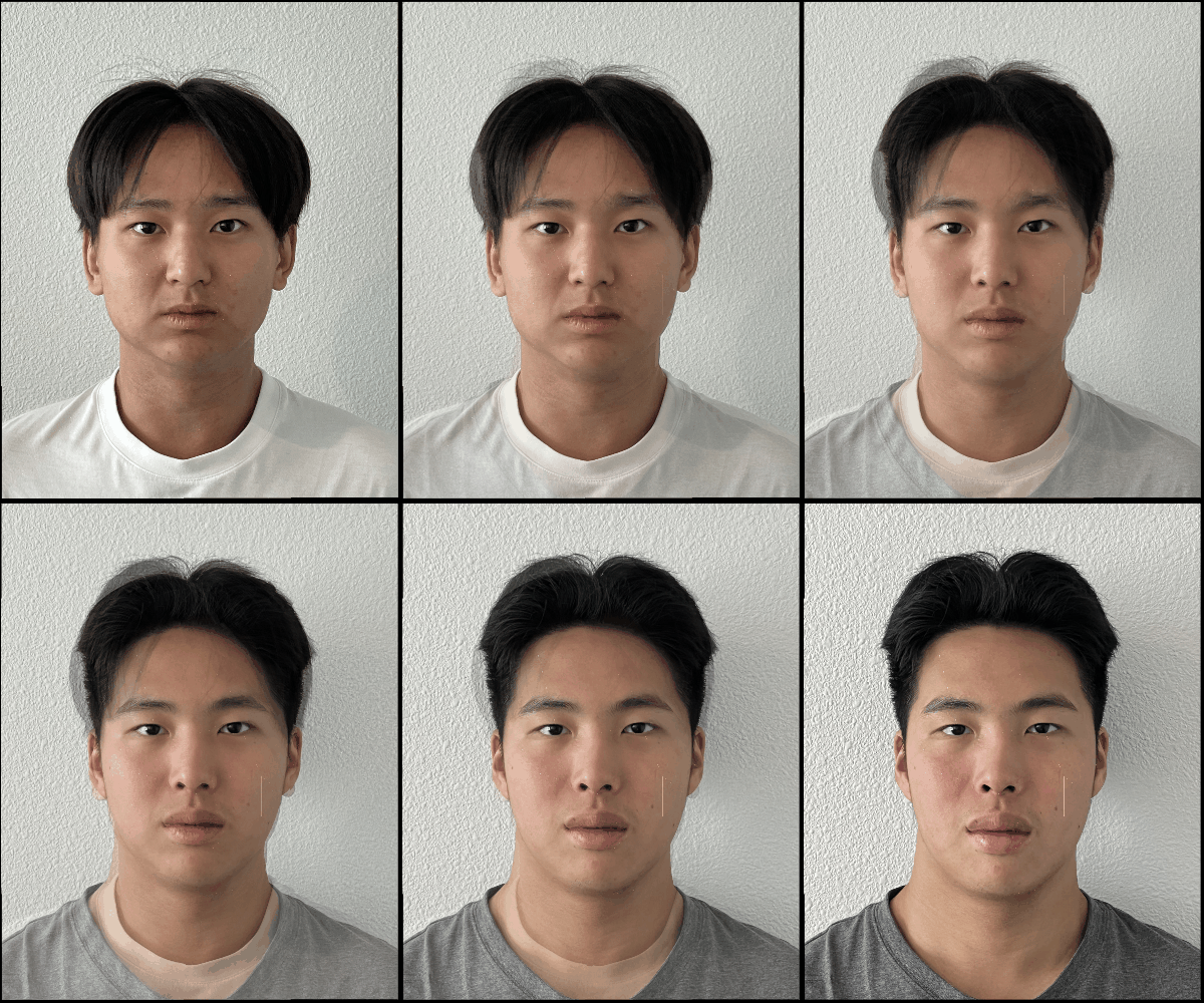
Figure 5: Morphed image with varying warp and dissolve fraction.

The mean face of a population

We now move on to morphing images to the mean face of a population. To compute the mean face, we used the IMM face dataset, which consists of 240 images of faces from different individuals. We calculate the mean face by first averaging the keypoints from all images, then warping each image to the mean geometry. Some examples are shown below.

Figure 6: Example warped images.

We then average the faces across all individuals. Before computing the mean face, we filter out all faces that are not front views. This process gives us the mean face, as shown in Figure 7. Since there are more males (128) than females (29) in the database, the resulting mean face resembles that of a male. To obtain a female mean face, we also restrict the set to include only female images.

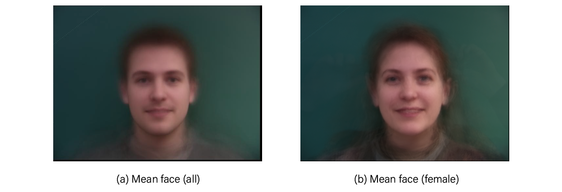
Figure 7: "Mean" face in the IMM face database. (a) All faces, (b) Restricted to female faces.

We can also warp images of our choice to the average geometry, as well as warp the average geometry to the images.

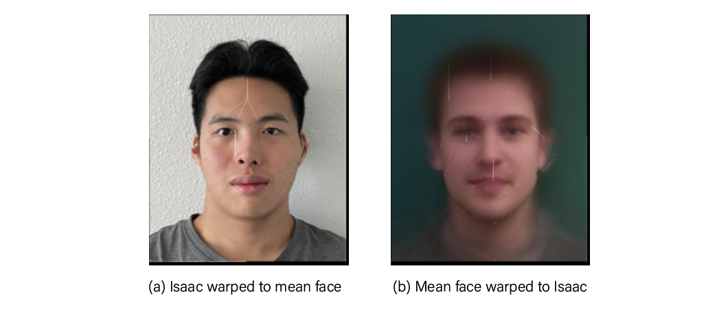
Figure 8: (a) Isaac warped to mean face, (b) The other way around.

Extrapolating from the mean

We can create a caricature from the mean by increasing the warp fraction $\alpha$ outside the range $[0,1]$. Below shows examples of warped Isaac with $\alpha=-0.1$ and $\alpha=2$, respectively.

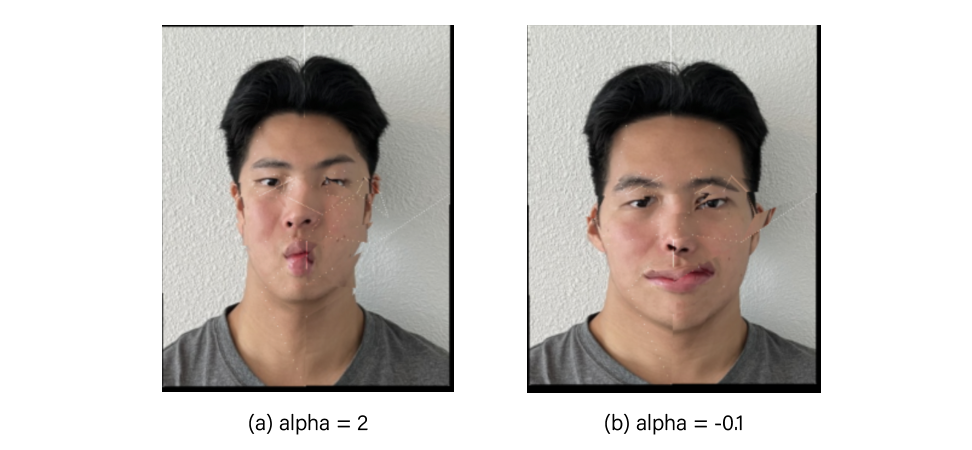
Figure 9: Isaacs with different features enhanced through varying $\alpha$.

Ethinicity change

We can use the mean image from a particular ethnic group to change the ethnicity of another face. For example, consider the mean face of Africans. After morphing the faces, we obtain the following results:

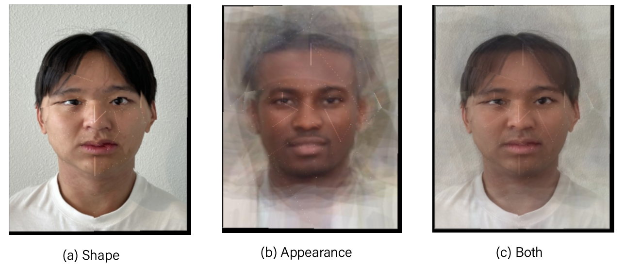
Figure 10: The shape (a), appearance (b), and morphed image (c).

The face becomes wider because two faces in the two images have different scale.

Principal componenent analysis

Another way to analyze faces is through PCA. Given a set of face images in a high-dimensional space, we can apply the standard PCA method to compress this space into a lower-dimensional span of important feature vectors. For simplicity, we used the grayscale FEI database, which has more aligned faces compared to the IMM face database. The first 20 eigenvectors of the image space are shown below.

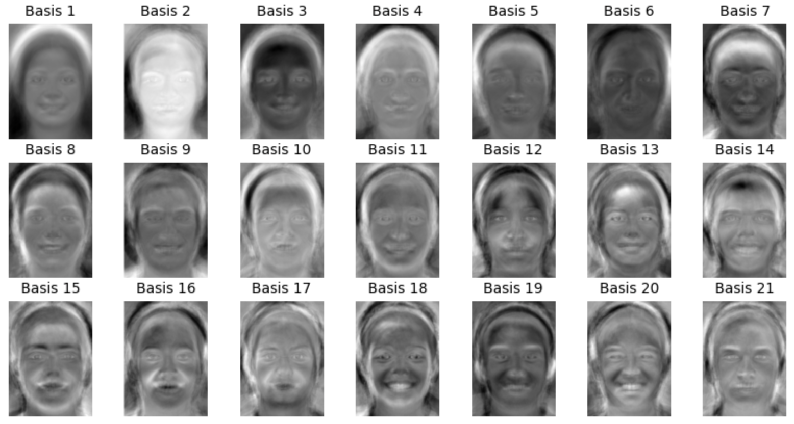
Figure 11: First 20 eigenfaces of the FEI face dataset.

These correspond to the characteristic features of faces in the dataset. Each face can be represented as a linear combination of these features. Some examples of reconstructed images are shown below.

Figure 12: Examples of reconstructed image by projecting to the span of eigenfaces.

We can emphasize certain features by adding more components of a basis face. For example, to make a face appear to smile, we can increase the weights of the basis faces associated with smiling expressions.

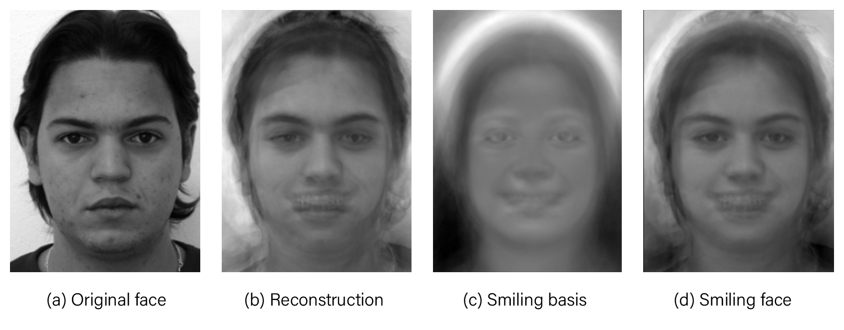
Figure 13: By increasing the effect of smiling eigenfaces (c), we can make the reconstructed image smile (d).