Project 2

Fun with Filters and Frequencies

Fun with filters

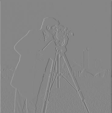
Convolution filters are one of the most fundamental operations in image processing, often used to extract or enhance local information within an image. One of the most common types is the gradient filter, defined as

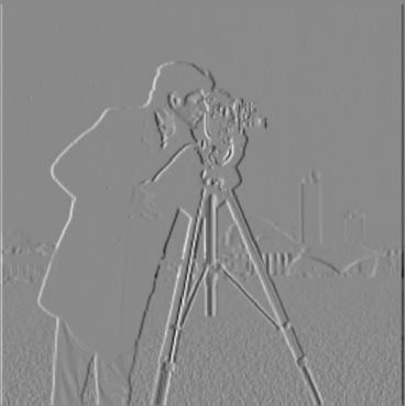
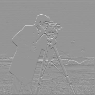
\[\mathbf{D}_x = \begin{bmatrix} -1 & 1 \\ \end{bmatrix} \hspace{20mm} \mathbf{D}_y= \begin{bmatrix} -1\\ 1 \end{bmatrix}\]

Note that the gradient filter is essentially a first-order approximation of the partial derivatives. When applied to an image, the filter captures edge information in both the $x$ and $y$ directions. Intuitively, the derivative signal is large when neighboring pixels differ significantly in intensity. We applied the gradient filter to the cameraman image, as shown below.

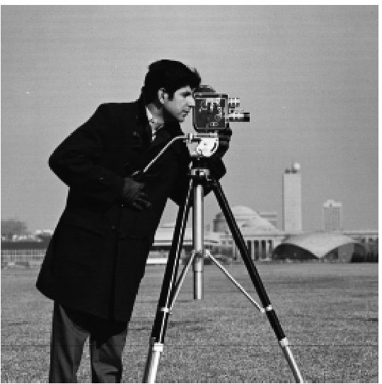
Original Image

Gradient in X direction

Gradient in Y direction

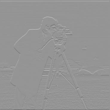
Figure 1: Cameran image and the estimated gradient.

We can also compute the magnitude and direction of the gradient, which are given by

\[\begin{align*} ||\nabla f||_2 &= \sqrt{\bigg(\frac{\partial f}{\partial x}\bigg)^2 + \bigg(\frac{\partial f}{\partial y}\bigg)^2}\\ \theta &= \tan^{-1}(\frac{\partial f}{\partial y}\bigg/\frac{\partial f}{\partial x}) \end{align*}\]

We see that the gradient magnitude extracts the edges in the image.

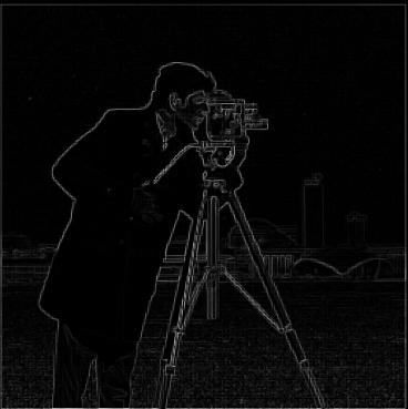
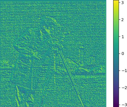
Figure 2: Gradient magnitude and direction.

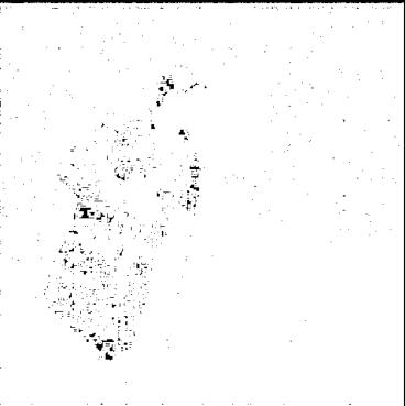
We can further filter out the edges by searching for a threshold $\tau$ and binarizing the gradient magnitude image through $|\nabla f|_2 \geq \tau$. Searching over $\tau \in (10^{-4}, 0.3)$, we find that $\tau = 0.1929$ gives us the clearest edges.

$\tau = 10^{-4}$

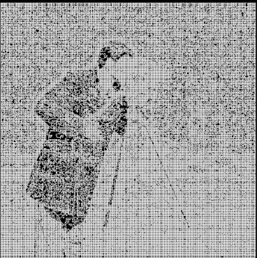
$\tau = 0.1929$

$\tau = 0.3$

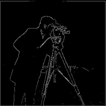
Figure 3: Edge detected from unblurred image.

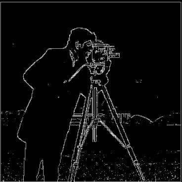
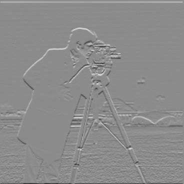
The extracted edge signal is weak due to the presence of high-frequency components in the image. To address this, we can first blur the image to remove these high-frequency components, then apply the gradient filter. Formally, we compute $\mathbf{D}_x \ast (G \ast f)$ and $\mathbf{D}_y \ast (G \ast f)$, where $G$ denote the Gaussian filter. Note that after blurring, we see a stronger edge signal in both the $x$ and $y$ direction.

Blurred gradient in X direction

Blurred gradient in Y direction

Blurred gradient magnitude

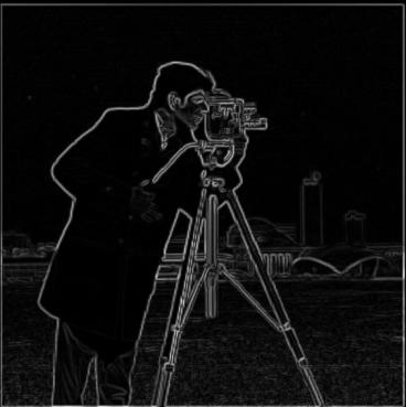
Figure 4: Blurred cameraman image by applying gradient operators on the blurred image.

Another way to perform the operation is to combine the derivative filter with the Gaussian filter, resulting in the derivative of Gaussian filter (DoG). This approach yields the same results.

Blurred gradient in X direction

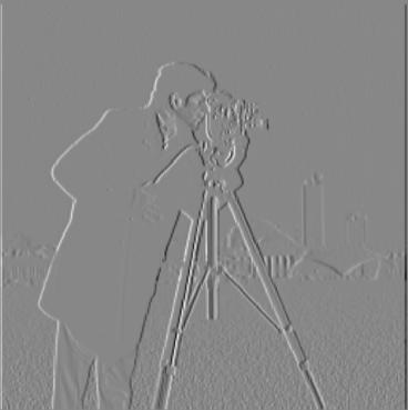
Blurred gradient in Y direction

Blurred gradient magnitude

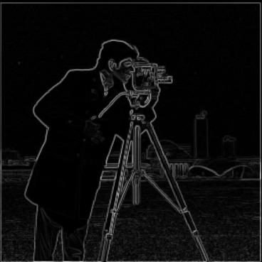
Figure 5: Blurred cameraman image by applying derivative of gradient operator.

Now, searching over the interval $\tau \in (10^{-4}, 0.1)$, we find that the optimal threshold $\tau=0.571$ produces much stronger edge responses.

$\tau=10^{-4}$

$\tau=0.571$

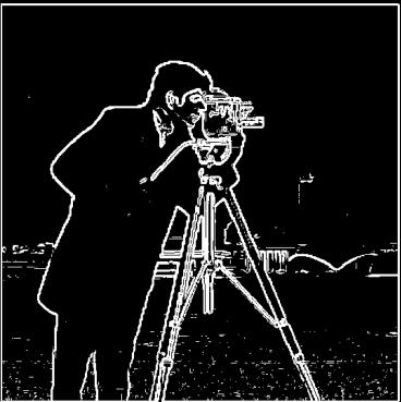
$\tau=0.1$

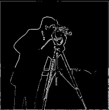
Figure 6: Edge detected from blurred image.

Fun with frequencies

In the previous section, we saw that removing high frequencies from an image can enhance edge detection. By manipulating high and low frequency components through the use of Gaussian filters, we can perform many interesting operations with images.

Image sharpening

One immediate application is image sharpening. An image appears sharper if it contains more high-frequency components $f_{high}$. This means that if we can extract the high-frequency components of the image, we can sharpen it by adding more of these components back. To extract the high-frequency component, we subtract the low-frequency component $f_{low}$ derived from the Gaussian filter, from the original image. We can combine this into a single filter as $I - G$, where $I$ denote the identity convolution. We extracted both components for the taj image.

Original image

Low resolution component

High resolution component

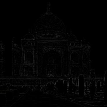
Figure 7: Extracted high and low frequency component from the image.

Now we can sharpen the original image by computing

\[f_{sharpened} = f + \alpha f_{high}\]

Where $\alpha\geq 0$ denote some scalar. We see that varying the scale $\alpha$ introduces different levels of details.

Unsharpened $\alpha=0$

$\alpha=1$

$\alpha=2$

$\alpha=3$

Figure 8: Varying the amount of high frequency component added.

We then apply this sharpening method to some images of our choice. For the following images, the $\alpha$ is set to be $3$.

❮ ❯

Figure 9: (Left) Original image, (Middle) Blurred image, (Right) Sharpened image with.

Hybrid images

We can also manipulate frequency to create hybrid images—images that change as a function of viewing distance. It has been observed that high frequency tends to dominate perception when the viewer is close, while low frequency dominates when the viewer is farther away. By blending both high and low frequency components from two different images, we can create hybrid images. In this section, we follow the approach of Olivia et al. The idea is to extract the low frequency from image 1 and the high frequency from image 2, and then average the results. Below, we present some results for grayscale images.

❮ ❯

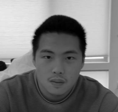
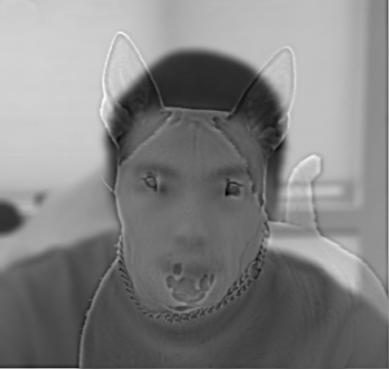
Figure 10: Hybrid image for grayscale images (Right).

The kernel size and standard deviation of the Gaussian filter used to separate the high and low-frequency components must be carefully tuned. Improper tuning can cause one image to overlap with the other, leading to failure.

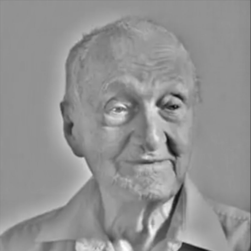
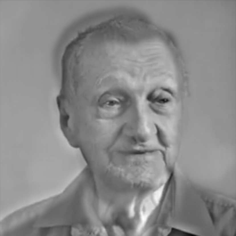
Figure 11: Extracted high and low frequency component from the image.

To understand the process of creating hybrid images, we can visualize the signal captured at each level using the Fast Fourier Transform (FFT). Note the attenuation of high-frequency components after blurring.

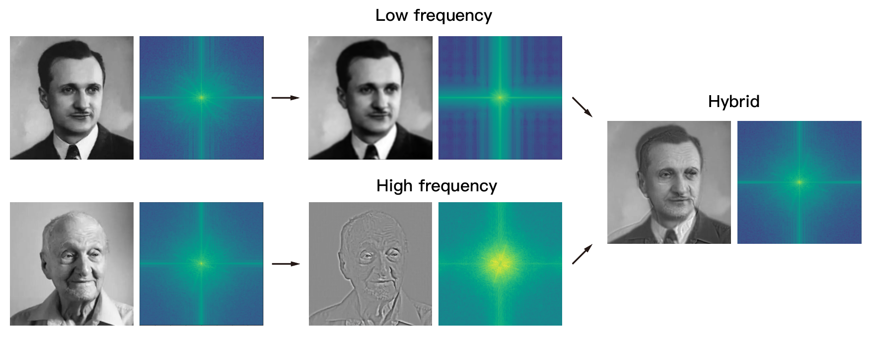
Figure 12: Fast Fourier transform analysis.

We can also apply the method to colored images. Below, we compare the effect of making different components grayscale. Regardless of whether the two images have a similar color profile or not, it seems that keeping both the high and low-frequency components colored gives better results. However, coloring the low-frequency component yields better results compared to coloring only the high-frequency component. This is because not much color is extracted from the high-frequency component, so the image appears grayscale if the background is not colored.

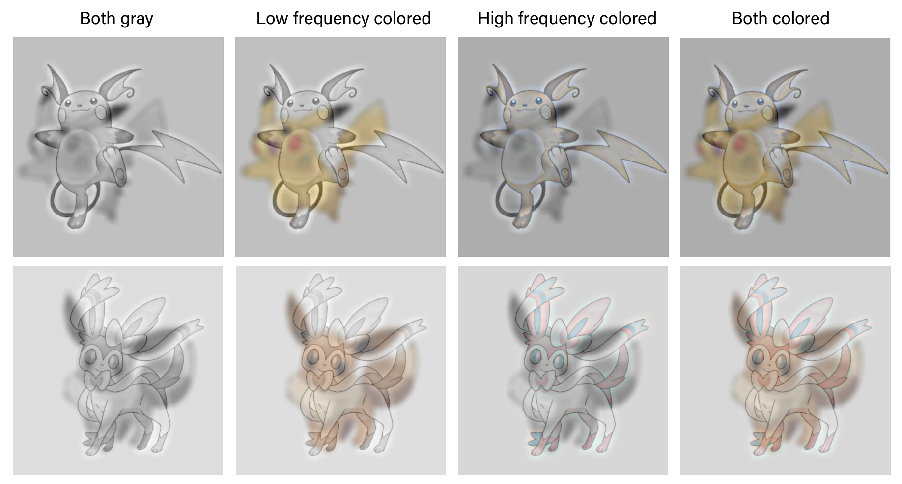
Figure 13: Comparison of hybrid images with different components colored.

Multiresolution blending

Another application of image frequency manipulation is image blending. The approach proposed by Burt and Adelson involves constructing a Laplacian pyramid for both images and then interpolating them across different levels. To obtain the final blended image, we sum all the levels in the Laplacian pyramid. Below is an example of blending an image of an orange and an apple (an oraple!). The interpolated image $f_i$ at each level can be expressed as

\[f_{i} = g_i * m_i + h_i * (1-m_i)\]

Where $g_i$ and $h_i$ represent the Laplacian stack images at level $i$ for two different images, and $m_i$ denotes the $i$th level of the binary mask in the Gaussian stack.

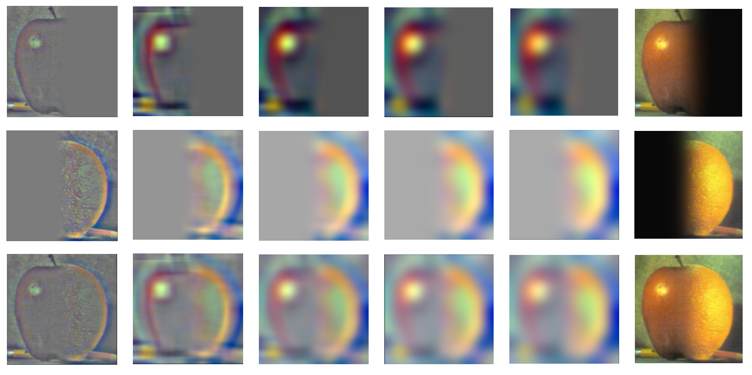
Figure 14: Laplacian pyramid for masked apple and orange.

We apply this method to a set of chosen images. On the left, the binary mask is displayed, and on the right, the resulting blended image is shown.

❮ ❯

Figure 15: Multiresolution blending results.