Radamacher Complexity

Introduction

From the previous blog, we see that the excess risk of the function class $\mathcal{F}$ can be bounded as follows

\[\begin{align*} R(\hat{f}) - R(f^*) &\leq 2\cdot \underbrace{\sup_{f\in \mathcal{F}}\lvert\hat{R}_n(f)-R(f)\rvert}_{\|\mathbb{P}_n-\mathbb{P}\|_{\mathcal{F}}} \end{align*}\]

To bound the excess risk, it suffices to control ${\left\lVert\mathbb{P}_n-\mathbb{P}\right\rVert} _{\mathcal{F}}$. In this blog, we will show that the term ${\left\lVert\mathbb{P}_n-\mathbb{P}\right\rVert} _{\mathcal{F}}$ is essentially controlled by the “complexity” of the function class $\mathcal{F}$, through two steps:

These two steps tells us that, with high probability, we can bound the excess risk by

\[R(\hat{f}) - R(f^*)\leq 2\mathcal{R}_n(\mathcal{F}) + \text{some extra term}\]

And in the final section, we will shift our focus to controlling the Rademacher complexity of different function classes.

A High Probability Bound

For the rest of the blog, we will assume that the function class is $b$-uniformly bounded, in other words, $\left\lvert f \right\rvert \leq b$ for all $f\in \mathcal{F}$. Under this assumption, it turns out ${\left\lVert\mathbb{P}_n-\mathbb{P}\right\rVert} _{\mathcal{F}}$ is sharply concentrated around its mean. We will argue this using the bounded difference inequality, this requires us to show that ${\left\lVert\mathbb{P}_n-\mathbb{P}\right\rVert} _{\mathcal{F}}$ satisfies the bounded differences property.

Theorem: Bounded Difference Inequality

Theorem (Bounded difference inequality): We say that $f:\mathbb{R}^n \rightarrow \mathbb{R}$ satisfy bounded difference property if there are constants $c_i\in \mathbb{R}$ such that $$|f(x_1, x_2, ..., x_i, ..., x_n) - f(x_1, x_2, ..., x_i', ..., x_n)| \leq c_i$$ For all $X_1, X_2,..., X_n$ and $X_i'$. If $f$ satisfies bounded difference property, then for any independent random variables $X_1, X_2,..., X_n$, we have $$\mathbb{P}[|f(X_1, X_2,..., X_n) - \mathbb{E}[f(X_1, X_2,..., X_n)]|\geq \epsilon] \leq \exp\bigg(-\frac{2\epsilon^2}{\sum_{i=1}^n c_i^2}\bigg)$$

To prove this, lets fix a sample $(x_1, x_2,.., x_n)$ and define:

\[h(x_1, x_2,..., x_n) = \lvert\hat{R}_n(f)-R(f)\rvert = \bigg|\frac{1}{n}\sum_{i=1}^n f(x_i) - \mathbb{E}[f(X)]\bigg|\]

So that

\[\|\mathbb{P}_n-\mathbb{P}\|_{\mathcal{F}} = \sup_{f\in \mathcal{F}} h(x_1, x_2,..., x_n)\]

Consider perturbing only the first sample coordinate from $x_1$ to $x_1’$, then

\[\begin{align*} h(x_1, x_2,..., x_n) - \sup_{f\in \mathcal{F}} h(x_1', x_2,..., x_n) &\leq h(x_1, x_2,..., x_n) - h(x_1', x_2,..., x_n)\\ &\leq \frac{1}{n}|f(x_1)-f(x_1')|\leq \frac{2b}{n} \end{align*}\]

Here, the second inequality follows from the reverse triangle inequality. Taking the supremum over all $f\in \mathcal{F}$, we conclude that ${\left\lVert\mathbb{P}_n-\mathbb{P}\right\rVert} _{\mathcal{F}}$ indeed satisfies a bounded difference condition with bound $2b/n$. Applying bounded difference inequality gives us

\[\|\mathbb{P}_n-\mathbb{P}\|_{\mathcal{F}} \leq \mathbb{E}[\|\mathbb{P}_n-\mathbb{P}\|_{\mathcal{F}}] + t \hspace{8mm}\text{with probability}\;1-\exp(-\frac{nt^2}{2b^2})\]

Or equivalently

\[\|\mathbb{P}_n-\mathbb{P}\|_{\mathcal{F}} \leq \mathbb{E}[\|\mathbb{P}_n-\mathbb{P}\|_{\mathcal{F}}] + b\sqrt{\frac{2\log(1/\delta)}{n}} \hspace{8mm}\text{with probability}\;1-\delta\]

This gives a probabilistic upper bound on the excess risk in terms of its expectation. We now proceed to bound the expectation.

Radamacher Complexity

The expectation is closely related to a complexity measure of the function class. This can be shown using a technique called symmetrization to bound the expectation. Let $Y_{1:n}$ be another sequence of i.i.d. random variables sampled from $\mathcal{X}$. Then

\[\begin{align*} \mathbb{E}[\|\mathbb{P}_n - \mathbb{P}\|_{\mathcal{F}}] &= \mathbb{E}_X\left[\sup_{f \in \mathcal{F}}\left|\frac{1}{n}\sum_{i=1}^n \Big(f(X_i) - \mathbb{E}[f(X)]\Big)\right|\right] \\ &= \mathbb{E}_X\left[\sup_{f \in \mathcal{F}}\left|\frac{1}{n}\sum_{i=1}^n \Big(f(X_i) - \mathbb{E}[f(Y_i)]\Big)\right|\right] \\ &\leq \mathbb{E}_{X, Y}\left[\sup_{f \in \mathcal{F}}\left|\frac{1}{n}\sum_{i=1}^n \Big(f(X_i) - f(Y_i)\Big)\right|\right] \end{align*}\]

In the second inequality, we used the fact that

\[\sup_{f\in \mathcal{F}} \mathbb{E}[f(X)] \leq \mathbb{E}_{X, \epsilon} [\sup_{f\in \mathcal{F}}|f(X)|]\]

Next, let $\epsilon_i$ be i.i.d. Rademacher random variables. Note that $f(X_i)-f(Y_i)$ has the same distribution as $\epsilon_i\bigl(f(X_i)-f(Y_i)\bigr)$. Therefore,

\[\begin{align*} \mathbb{E}[\|\mathbb{P}_n - \mathbb{P}\|_{\mathcal{F}}] &\leq \mathbb{E}_{X, Y, \epsilon}\left[\sup_{f \in \mathcal{F}}\left|\frac{1}{n}\sum_{i=1}^n \epsilon_i\bigl(f(X_i) - f(Y_i)\bigr)\right|\right] \\ &\leq 2\,\mathbb{E}\left[\sup_{f \in \mathcal{F}}\left|\frac{1}{n}\sum_{i=1}^n \epsilon_i f(X_i)\right|\right] \end{align*}\]

The quantity

\[\mathcal{R}_n(\mathcal{F}) = \mathbb{E}_{X, \epsilon}\left[\sup_{f \in \mathcal{F}}\left|\frac{1}{n}\sum_{i=1}^n \epsilon_i f(X_i)\right|\right]\]

is called the Rademacher complexity of the function class $\mathcal{F}$. This can be interpreted as a measure of the size of the function class. The reasoning is as follows: suppose we are given a sample $x_{1:n}$, and for each sample we randomly assign a label $\epsilon_i \in \lbrace \pm 1 \rbrace$ by flipping a fair coin. Given a binary valued function $f \in \mathcal{F}$, we can measure how well it fits the random labels by evaluating the inner product

\[\text{success rate} = \frac{1}{n}\sum_{i=1}^n \epsilon_i f(x_i),\]

Which is large only when $f$ consistently output the same sign as the label.

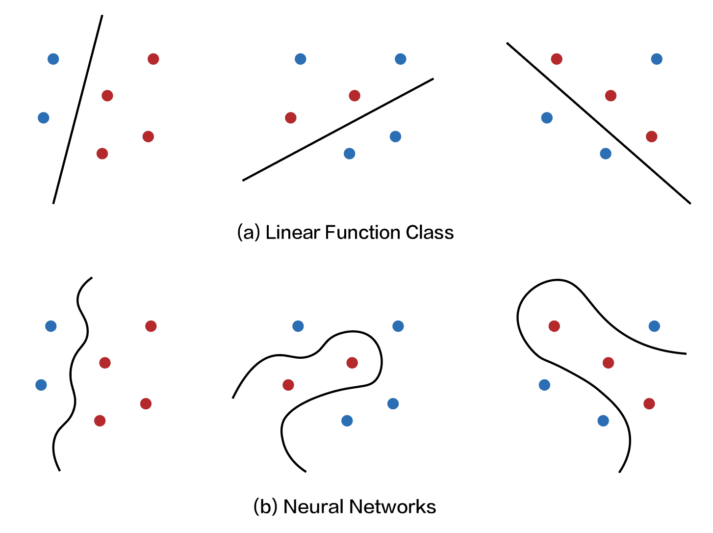
So when the Radamacher complexity is high, this means that on average, given any dataset $x_{1:n}$ and random labels $\lbrace \epsilon_i \rbrace _{i \in [n]}$, we can always find a function $f \in \mathcal{F}$ that fits the data well. Naturally, a function class with limited representation power (e.g., the set of all linear functions) should have lower Rademacher complexity than function classes with rich representation power (e.g. a neural network).

What we’ve shown is that the excess risk is essentially controlled by the representation power of the function class, which makes sense since a smaller function class is less likely to interpolate or overfit the data and should generalize better. The next step, of course, is to further bound the Radamacher complexity of a given function class.

Bounding the Radamacher complexity

We now focus on controlling the Rademacher complexity for different function classes. In some cases, it’s possible to obtain bounds directly using standard tools like Jensen inequality or Cauchy Schwarz inequality (see example below).

Example: Radamacher complexity of Linear Classifiers

Consider the set of linear classifiers with bounded weights: $$\mathcal{F}=\{f(x)=\langle w, x\rangle:\|w\|_2\leq B, \|x\|_2\leq R\}$$ The Radamacher complexity is given by $$ \begin{align*} \mathcal{R}_n(\mathcal{F}) &= \mathbb{E}_{X_{1:n}, \epsilon_{1:n}}\bigg[\sup_{f\in \mathcal{F}} \frac{1}{n}\sum_{i=1}^n \epsilon_i \langle w, X_i\rangle\bigg] \\ &\leq \mathbb{E}_{X_{1:n}, \epsilon_{1:n}}\bigg[\sup_{\|w\|_2\leq B} \frac{1}{n}\|w\|_2 \cdot \bigg\|\sum_{i=1}^n \epsilon_i X_i\bigg\|_2\bigg] \\ &\leq \frac{B}{n} \mathbb{E}_{X_{1:n}, \epsilon_{1:n}}\bigg[\bigg\|\sum_{i=1}^n \epsilon_i X_i\bigg\|_2\bigg] \\ &\leq \frac{B}{n} \sqrt{\mathbb{E}_{X_{1:n}, \epsilon_{1:n}}\bigg[\sum_{i, j=1}^n \epsilon_i \epsilon_j \langle X_i, X_j \rangle\bigg]} \\ \end{align*} $$ Finally, note that for $i\neq j$, $\mathbb{E}[\epsilon_i \epsilon_j]=0$ by independence, so it suffice considering the cases where $i=j$: $$ \begin{align*} \mathcal{R}_n(\mathcal{F}) &\leq \frac{B}{n}\sqrt{\mathbb{E}_{X_{1:n}} \bigg[\sum_{i=1}^n \|X_i\|_2^2\bigg]} \\ &\leq \frac{B}{n}\cdot \sqrt{n} R \\ &= \frac{BR}{\sqrt{n}} \end{align*} $$

Here, we focus on general techniques for controlling the Rademacher complexity. To begin, we introduce the notion of “size” of a function class $\mathcal{F}$. Given a fixed sample $x_{1:n}$, we define:

\[\mathcal{F}(x_{1:n}) = \{(f(x_1), f(x_2), \ldots, f(x_n)) \mid f \in \mathcal{F}\}\]

This set captures all the distinct ways that functions in $\mathcal{F}$ can behave on the sample. The “size” of $\mathcal{F}$ is then defined as the size of the maximum number of such distinct outputs over all possible samples:

\[|\mathcal{F}|= \sup_{x_{1:n}} |\mathcal{F}(x_{1:n})|\]

Different techniques are used to bound the Rademacher complexity depending on whether $\lvert \mathcal{F} \rvert$ is finite or not:

• If $\lvert\mathcal{F}(x_{1:n})\rvert < \infty$: Apply maximal inequality and VC theory.
• If $\lvert\mathcal{F}(x_{1:n})\rvert = \infty$: Apply discretization and metric entropy methods.

For the remainder of this blog, we will assume that $\lvert\mathcal{F}(x_{1:n})\rvert < \infty$ and leave the other case to the next blog.

Maximal Inequality Bounds

When $\lvert\mathcal{F}(x_{1:n})\rvert < \infty$, we can bound the Rademacher complexity using maximal inequality. We start by rewriting the definition as conditional expectation:

\[\mathcal{R}_n(\mathcal{F}) = \mathbb{E}_{X, \epsilon}\left[\sup_{f \in \mathcal{F}} \left|\frac{1}{n}\sum_{i=1}^n \epsilon_i f(X_i)\right|\right]= \mathbb{E}_X\left[\mathbb{E}_\epsilon\left[\sup_{v \in \mathcal{F}(X_{1:n})} \left|\frac{1}{n} \langle v, \epsilon \rangle\right| \,\bigg|\, X\right]\right]\]

Note that $\langle v, \epsilon \rangle / n$ is sub-Gaussian. This is because $\epsilon_i$ are Rademacher random variables (sub-Gaussian with parameter $1$), so

\[\frac{\langle v, \epsilon \rangle}{n} = \frac{1}{n}\sum_{i=1}^n v_i\epsilon_i\sim SG(\frac{1}{n}\|v\|_2)\]

We can find a common sub-Gaussian parameter by taking supremum over the samples:

\[\sigma_n = \sup_{v \in \mathcal{F}(X_{1:n})} \frac{1}{n} \|v\|_2 = \sup_{f \in \mathcal{F}} \frac{1}{n} \sqrt{\sum_{i=1}^n f(X_i)^2}\]

Next, since $\lvert\mathcal{F}(x_{1:n})\rvert < \infty$, applying maximal inequality, we see that the conditional expectation is bounded by:

\[\mathbb{E}_\epsilon\left[\sup_{v \in \mathcal{F}(X_{1:n})} \left|\frac{1}{n} \langle v, \epsilon \rangle\right| \,\bigg|\, X_{1:n}\right] \leq \sigma_n \sqrt{2\log \big(2|\mathcal{F}(X_{1:n})|\big)}\]

Further taking expectation over $X$, we have:

\[\begin{align*} \mathcal{R}_n(\mathcal{F}) &\leq \mathbb{E}_X\left[\sqrt{\frac{1}{n} \sum_{i=1}^n f(X_i)^2} \cdot \sqrt{\frac{2 \log \big(2|\mathcal{F}(X_{1:n})|\big)}{n}}\right]\\ &\leq \mathbb{E}_X\left[\sqrt{\frac{1}{n} \sum_{i=1}^n f(X_i)^2}\right] \cdot \sqrt{\frac{2 \log \big(2|\mathcal{F}|\big)}{n}}\\ &\lesssim \sqrt{\frac{2\log \big(2|\mathcal{F}|\big)}{n}} \end{align*}\]

This tells us that the Radamacher complexity is approximately controlled by $\lvert \mathcal{F} \rvert$. The behavior of the bound changes depending on how $\lvert \mathcal{F} \rvert$ scales with $n$.

Vapnik-Chervonenkis Theory

Consider the case of binary classification, so that $f:\mathcal{X}\rightarrow \lbrace \pm 1\rbrace$. In the worst case, $\lvert\mathcal{F}\rvert = 2^n$ grows exponentially with $n$, so the bound becomes:

\[\mathcal{R}_n(\mathcal{F})\lesssim \sqrt{\frac{2\log \big(2|\mathcal{F}|\big)}{n}}=\sqrt{\frac{2(n+1)\log 2}{n}}\]

Which does not converge to 0 as $n \to \infty$. This means that no matter how many samples we use, we cannot guarantee the excess risk will be small! On the other hand, suppose that $\lvert\mathcal{F}\rvert$ grows at most polynomially, i.e., $\lvert\mathcal{F}\rvert \leq (n+1)^\nu$ for some $\nu$. Then we have:

\[\mathcal{R}_n(\mathcal{F})\lesssim \sqrt{\frac{2\log \big(2|\mathcal{F}|\big)}{n}}=\sqrt{\frac{2\nu \log (n+1)}{n}}\rightarrow 0 \text{ as } n\to\infty\]

This suggests that as long as $\lvert\mathcal{F}\rvert$ has polynomial growth, we can ensure that the excess risk goes to zero given enough samples. But what kinds of function classes have polynomial size? This question is addressed by Vapnik–Chervonenkis (VC) theory through the concept of VC dimension.

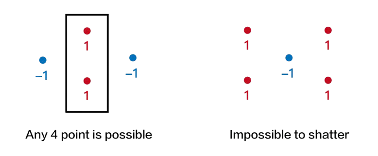
Suppose $f: \mathcal{X} \rightarrow \lbrace \pm 1\rbrace$ is a binary-valued function. We say that the set $X_{1:n}$ is shattered by $\mathcal{F}$ if $\lvert\mathcal{F}(x_{1:n})\rvert = 2^n$. In other words, no matter how we assign binary labels to the samples in $X_{1:n}$, there exists a function $f \in \mathcal{F}$ that can perfectly classify all of them. The VC dimension $\nu(\mathcal{F})$ is defined as the largest integer $n$ such that there exists a set $X_{1:n}$ shattered by $\mathcal{F}$.

Examples of VC dimension

Example 1 (Open intervals): Consider the set of indicator functions for half-intervals on the real line $$\mathcal{A} = \{\mathbb{1}\{x\in (-\infty, a]\}: a\in \mathbb{R}\}$$ The VC dimension is $1$, since it's impossible to shatter $2$ points using half intervals.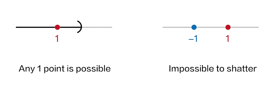

Example 2 (Rectangles): Consider the set of indicator functions on rectangles in $\mathbb{R}^2$. $$\mathcal{R} = \{\mathbb{1}\{x\in [a, b]\times [c, d]\}: a, b, c, d\in \mathbb{R}\}$$ The VC dimension is $4$, since it's always possible to shatter $4$ points but impossible to shatter $5$ points.

Example 3 (Linear Classifiers): Consider the set of linear classifiers in $n$ dimensions $$\mathcal{F} = \{f: f(\mathbf{x})=\text{sign}(\mathbf{w}^T\mathbf{x}), \mathbf{w}\in \mathbb{R}^n\}$$ The VC dimension is $n$. Given any $\leq n$ points, the system $\mathbf{X}\mathbf{w}=\mathbf{y}$ always has a solution, and therefore $\text{sign}(\mathbf{X}\mathbf{w})=\mathbf{y}$. This proves that the functions can shatter $n+1$ points. We now show that there exists $n+1$ points such that it cannot be shattered. Given any $\mathbf{x}_1, \mathbf{x}_2,..., \mathbf{x}_{n+1}\in \mathbb{R}^n$, these vectors are linearly dependent. WLOG, suppose $$\mathbf{x}_{n+1} = \sum_{i=1}^n \alpha_i \mathbf{x}_{i}$$ such that not all $\alpha_i$ are $0$. Set $y_{n+1}=-1$ and $y_i=\text{sign}(a_i)$ for all $i\leq n$. Suppose there exists $\mathbf{w}$ that classifies the first $n$ points correctly, so $y_i=\text{sign}(\mathbf{w}^T\mathbf{x}_i)$. Then $$\text{sign}(\mathbf{w}^T \mathbf{x}_{n+1}) = \text{sign}\bigg(\sum_{i=1}^n \alpha_i \mathbf{w}^T\mathbf{x}_{i}\bigg) > 0 \neq y_{n+1}$$ This gives us an instance of points that cannot be shattered by the function class, so the VC dimension is $n$.

From this definition, it’s clear that the VC dimension is closely related to model complexity. A larger VC dimension implies that the function class $\mathcal{F}$ can correctly classify more configurations of points, which indicates greater expressiveness. This relationship is formalized by a foundational result, proven independently by Vapnik and Chervonenkis in 1971, by Sauer in 1972, and by Shelah also in 1972:

Theorem (Vapnik-Chervonenkis, Sauer-Shelah): If $\mathcal{F}$ has VC-dimension of $\nu$, then

\[\sup_{X_{1:n}} |\mathcal{F}(X_{1:n})|\leq \sum_{i=1}^\nu {n\choose i}\leq \min\{(n+1)^\nu, \bigg(\frac{ne}{\nu}\bigg)^\nu\}\]

This theorem immediately gives us the following bound on the Rademacher complexity:

\[\mathcal{R}_n(\mathcal{F})\lesssim \sqrt{\frac{2\nu(\mathcal{F}) \log (n+1)}{n}}\]